Section 1: Understanding Irregular and Asynchronous Data
Why Traditional Time-Series Models Assume Regular Intervals
Traditional sequence models generally process observations as an ordered series of discrete steps. For example, a time-series dataset might contain temperature measurements recorded every five minutes. Each observation is assigned a position in the sequence, and the model learns how the values evolve from one position to the next.
A regularly sampled sequence can be represented as:
[
X = {x_1,x_2,\ldots,x_T}
]
where (x_t) represents an observation at sequence position (t). In a regular dataset, the time difference between consecutive observations is constant:
[
t_{i+1}-t_i=\Delta t
]
This assumption simplifies model design. A recurrent neural network can update its hidden state once per observation, while a temporal convolutional network can apply filters across equally spaced positions. A transformer can use positional information to represent sequence order.
The difficulty appears when observations are not equally spaced.
Consider a monitoring system that records a machine's vibration level at the following times: 09:00:00, 09:00:02, 09:00:03, 09:00:18, and 09:01:10. The first three observations arrive close together, but the remaining intervals are substantially longer.
If the model processes these observations as five equally spaced sequence positions, it may interpret the temporal distance between every pair of observations as equivalent. That is incorrect. The system had only one second between the second and third observations but 52 seconds between the fourth and fifth.
The elapsed time can contain important information. A sudden change after a long period of stability may have a different interpretation from the same change occurring immediately after another measurement. In financial systems, a cluster of transactions within a few seconds may signal different behavior from the same number of transactions spread across an hour.
Traditional models can incorporate elapsed time as an additional feature, but this does not necessarily provide a principled representation of the underlying continuous process. The model still advances through discrete observation steps, and the effect of elapsed time must be learned through the input representation.
Continuous-time modeling provides a more direct alternative. It defines how a hidden state evolves as time passes, allowing the model to account for the actual interval between observations rather than treating every sequence position as an equivalent time step.
What Makes Data Irregular and Asynchronous?
Irregular data describes observations recorded at non-uniform time intervals. The time difference between consecutive measurements varies rather than following a fixed schedule.
Asynchronous data refers to observations from different sources that do not necessarily arrive or occur at the same time. A system may receive measurements from several sensors, databases, services, or event streams, each operating on a different schedule.
These concepts frequently occur together, but they are not identical. A single sensor can produce irregularly sampled data, while multiple sensors can produce asynchronous observations even if each individual sensor operates at a regular frequency.
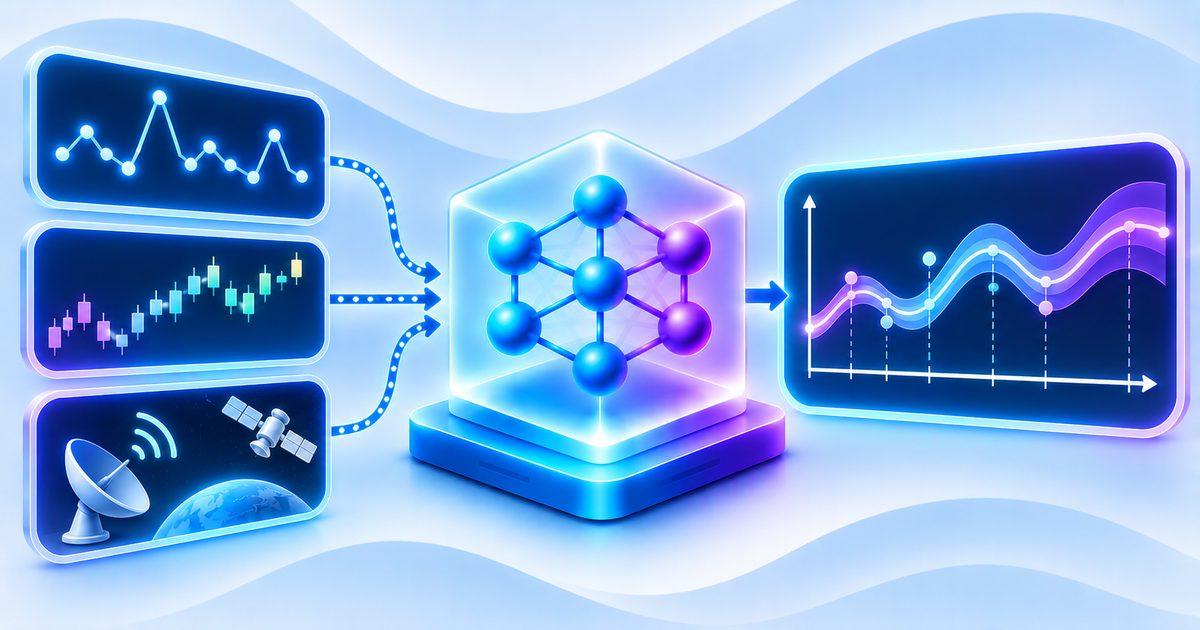
Consider an industrial monitoring platform with three data sources. A vibration sensor records measurements every 100 milliseconds. A temperature sensor sends an update every 10 seconds. A maintenance system produces an event only when an operator records an inspection or repair.
The system does not receive one synchronized observation containing all three values. Instead, it receives separate events at different times. A machine learning model must combine the available information without assuming that every source has a measurement at every time point.
The problem can be represented as a collection of time-stamped observations:
[
D={(t_i,x_i,m_i)}_{i=1}^{N}
]
Here, (t_i) is the observation time, (x_i) is the observed value, and (m_i) identifies the variable or data source associated with that observation.
In multivariate settings, each variable may have its own observation schedule. Some features may be available frequently, while others may be missing for long periods. A model must therefore account for both temporal irregularity and variable-level observation availability.
There is also an important distinction between event time and arrival time. Event time represents when something actually happened, while arrival time represents when the system received the corresponding record. Distributed systems may introduce network delays, buffering, retries, and out-of-order delivery. A continuous-time model that uses incorrect timestamps can learn misleading temporal relationships.
Engineers should preserve source timestamps, define how late-arriving events are handled, and distinguish missing observations from delayed observations. These decisions are part of the modeling problem rather than merely data-engineering details.
Why Missing Values and Observation Timing Carry Information
Missing values are often treated as a preprocessing problem. Engineers may replace them with the mean, forward-fill previous measurements, interpolate between known values, or remove incomplete records.
These approaches can be useful, but missingness itself may contain information about the system.
In healthcare, a measurement may be recorded more frequently when a patient's condition becomes unstable. A patient who requires repeated blood tests may have a different clinical context from one whose measurements remain stable. The frequency of observation can therefore be associated with the underlying state.
In industrial monitoring, a sensor may transmit additional readings when an anomaly is detected. In financial services, transaction frequency may change when customer behavior changes. In application monitoring, an increase in error events may cause logging systems to generate more records.
This means that the observation process can be informative.
A complete representation of irregular time-series data may need to include three types of information: the observed value, the time at which it was observed, and whether the observation was available at that time.
A common approach is to use a value mask:
[
m_{t,j}=
\begin{cases}
1, & \text{if variable }j\text{ is observed at time }t\
0, & \text{otherwise}
\end{cases}
]
The mask indicates which measurements are available. Engineers may also include time-since-last-observation features:
[
\delta_{t,j}=t-t_{\text{last observed},j}
]
This provides the model with information about how long a variable has gone without a new measurement.
However, missingness should not automatically be interpreted as evidence of a particular outcome. A sensor may stop reporting because of a network failure rather than because the monitored machine has changed state. A clinical measurement may be absent because of workflow decisions rather than patient physiology.
The model should distinguish between the data-generating process and the observation process. When observation timing is informative, it can be included in the model. When it is driven by external operational failures, it may need to be handled as a separate reliability signal.
The relationship between data quality and temporal structure becomes especially important when building reliable pipelines. Teams can draw on practices described in "ML Data Pipelines for Software Engineers: From Event Streams to Model-Ready Data" to preserve timestamps, track missingness, and create consistent model-ready representations without discarding useful event information.
Key Takeaway
Irregular and asynchronous data cannot always be represented faithfully as equally spaced sequences. Observation timing, missingness, and differences between data sources may contain important information about the underlying process. Continuous-time machine learning provides a framework for modeling these relationships by representing hidden-state evolution as a function of real-valued time. Its value is greatest when elapsed time and event timing materially influence the prediction task.
Section 2: Core Architectures for Continuous-Time Machine Learning
Neural Ordinary Differential Equations
Neural Ordinary Differential Equations provide one of the foundational architectures for continuous-time machine learning. Instead of updating a hidden state through a fixed sequence of discrete transformations, a Neural ODE defines how that state changes continuously over time.
The central formulation is:
[
\frac{dh(t)}{dt}=f_\theta(h(t),t)
]
Here, (h(t)) represents the hidden state at time (t), and (f_\theta) is a neural network that defines the derivative of the hidden state.
The state at a later time can be obtained by solving the differential equation:
[
h(t_1)=h(t_0)+
\int_{t_0}^{t_1}f_\theta(h(t),t),dt
]
Instead of learning one transformation for each sequence position, the model learns a continuous vector field that determines how the hidden representation evolves.
This is useful for irregular data because the model can integrate the hidden state across the actual time interval between observations. A gap of one second and a gap of one hour are handled as different integration intervals.
Neural ODEs typically rely on numerical solvers such as adaptive Runge-Kutta methods. These solvers estimate the trajectory by evaluating the learned derivative function at selected points. The solver can adjust its step size according to the numerical error tolerance.
This flexibility introduces an important engineering trade-off. Adaptive solvers can provide accurate approximations, but the number of function evaluations may vary depending on the dynamics. Complex trajectories may require more computational work than smooth ones.
Training also requires gradients through the differential equation solver. The adjoint sensitivity method is one approach used to reduce memory requirements during backpropagation, although its numerical behavior and accuracy must be considered carefully.
Neural ODEs are useful when a continuous latent process is an appropriate representation of the problem. However, a basic Neural ODE has a limitation: its trajectory is determined by its initial condition and learned dynamics. It does not automatically incorporate new observations after the initial state has been established.
This is one reason why ODE-RNNs and Neural CDEs are important extensions for irregularly sampled data.
The original Neural ODE work introduced the idea of parameterizing continuous-depth neural networks using differential equations. Its formulation established a foundation for later research into continuous-time latent dynamics and irregular time-series modeling.
ODE-RNNs and Latent ODE Models
ODE-RNNs combine continuous-time state evolution with discrete observation updates. Between observations, the hidden state evolves according to a differential equation. When a new observation arrives, a recurrent update incorporates the measurement.
A simplified process can be written as:
[
h(t_i^-)=
\operatorname{ODESolve}
\left(f_\theta,h(t_{i-1}^+),t_{i-1},t_i\right)
]
[
h(t_i^+)=
\operatorname{RNNUpdate}(h(t_i^-),x_i)
]
The notation (t_i^-) represents the state immediately before incorporating the new observation, while (t_i^+) represents the state immediately afterward.
This architecture captures two different processes. The differential equation describes how the system evolves between measurements, while the recurrent update describes how new information changes the hidden state.
Latent ODE models extend this idea by learning a continuous trajectory in a latent space. An encoder processes observed data and estimates an initial latent state or a distribution over latent states. A Neural ODE then evolves that representation over time, and a decoder maps the latent trajectory back into the observation space.
This architecture can support reconstruction, interpolation, extrapolation, and probabilistic modeling of irregular time series.
The original Latent ODE research by Rubanova, Chen, and Duvenaud introduced ODE-RNNs and Latent ODEs for irregularly sampled time-series data. It also demonstrated how observation times can be modeled using a Poisson process, allowing the model to represent not only the measured values but also the timing of observations.
The ability to model observation times is significant because the timing process may contain information about the underlying system. For example, an increase in measurement frequency may correspond to a change in operational conditions.
However, the observation process must be interpreted carefully. A learned Poisson process may capture correlations between measurement frequency and system state, but it does not automatically establish why those measurements occurred.
ODE-RNN and Latent ODE models are especially relevant when observations arrive at irregular intervals and the model needs to maintain a continuously evolving representation between updates.
Neural SDEs, Continuous Recurrent Units, and Hybrid Models
Not every real-world process evolves deterministically. Many systems contain stochastic variation caused by environmental uncertainty, measurement noise, random events, or unobserved influences.
Neural Stochastic Differential Equations extend continuous-time modeling by incorporating a stochastic component into the state dynamics.
A general formulation is:
[
dh(t)=f_\theta(h(t),t),dt+
g_\theta(h(t),t),dW(t)
]
Here, (f_\theta) represents the drift function, (g_\theta) represents the diffusion function, and (W(t)) is a stochastic process, commonly modeled using Brownian motion.
The drift component describes the expected direction of state evolution, while the diffusion component represents stochastic variation.
This is useful when the objective is to model uncertain trajectories rather than one deterministic path. Financial systems, biological processes, and physical systems with noisy dynamics may benefit from this formulation.
However, stochastic differential equations introduce additional computational and numerical challenges. Training requires methods for handling stochastic trajectories and estimating gradients through stochastic processes. The choice of numerical scheme can also influence stability.
Continuous Recurrent Units provide another approach. Rather than relying on a general-purpose numerical ODE solver for every state transition, CRUs use structured continuous-time state-space dynamics and filtering techniques to process irregular observations.
The CRU research demonstrates how continuous-discrete filtering can support irregular time-series modeling while avoiding some of the numerical integration overhead associated with general Neural ODE architectures.
Hybrid architectures combine continuous-time evolution with discrete event updates, recurrent mechanisms, attention, or state-space components. These designs can be useful when the underlying system evolves continuously but also experiences sudden events or observations that cause abrupt state changes.
A machine may operate continuously while receiving discrete maintenance events. A patient may experience continuous physiological changes while undergoing occasional interventions. A financial system may evolve continuously in some respects while reacting to discrete transactions or policy events.
The choice of architecture should reflect the process being modeled. Deterministic Neural ODEs, observation-driven Neural CDEs, stochastic Neural SDEs, and structured continuous recurrent models offer different assumptions and computational trade-offs.
Continuous-time models also introduce production considerations that extend beyond selecting an appropriate neural architecture. Their inference workflows may involve numerical integration, interpolation, event-time processing, and additional computation when observations arrive irregularly. These operations must be evaluated against practical requirements such as prediction latency, throughput, memory consumption, and computational cost. Engineers moving these models from experimentation into production can benefit from the principles discussed in “From Notebook to Low-Latency Service: The Engineering Journey of a Production ML Model”, particularly the importance of profiling the complete inference pipeline, optimizing preprocessing, and validating performance under realistic workloads.
Key Takeaway
Continuous-time machine learning includes several complementary architectures. Neural ODEs model continuous hidden-state evolution, ODE-RNNs combine continuous dynamics with discrete observation updates, Latent ODEs represent continuous trajectories in latent space, and Neural CDEs allow irregular observations to control the hidden state. Neural SDEs and Continuous Recurrent Units extend the framework to stochastic or computationally structured dynamics. Architecture selection should reflect the behavior of the underlying process and the available computational budget.
Section 3: Engineering Challenges and Production Deployment
Numerical Integration, Computational Cost, and Model Scalability
Continuous-time models introduce computational requirements that differ from conventional discrete-time networks.
A Neural ODE or Neural CDE typically requires numerical integration to estimate the hidden-state trajectory. The solver evaluates a learned derivative function at selected time points and uses those evaluations to approximate the solution.
The computational cost depends on several factors, including the length of the observation interval, the complexity of the learned dynamics, solver tolerances, hidden-state dimensionality, and the number of function evaluations.
Adaptive solvers can use larger steps when the trajectory is smooth and smaller steps when it changes rapidly. This improves numerical flexibility, but it can also make inference latency less predictable.
For real-time systems, unpredictable solver execution time can be a serious problem. An autonomous system may have a strict deadline for producing a control update. A healthcare monitoring system may need to generate a prediction within a specified response window.
Training introduces additional overhead because gradients must be computed through the continuous dynamics. Adjoint methods can reduce memory requirements, but they involve their own numerical considerations.
One alternative is to use structured continuous-time architectures that have more efficient or closed-form state transitions. Continuous Recurrent Units are an example of an approach designed to reduce some of the computational cost associated with general numerical ODE solvers.
Engineers should benchmark the complete model rather than evaluating only its prediction accuracy. Important measurements include inference latency, solver function evaluations, memory usage, throughput, energy consumption, and numerical stability.
The architecture should be selected based on the deployment environment. A research model running on a GPU cluster may tolerate a more expensive solver than an embedded device or real-time control system.
Continuous-time modeling should provide a measurable advantage over simpler alternatives. If a time-aware recurrent network or a conventional transformer produces similar predictive quality with substantially lower latency, it may be the better engineering choice.
Missing Data, Timestamp Quality, and Asynchronous Event Processing
Continuous-time models require accurate temporal information. If timestamps are inconsistent or incorrect, the model may learn misleading dynamics.
Distributed systems introduce several timing problems. Events may arrive late because of network latency. Messages may be delivered out of order. Different sensors may use clocks with different levels of precision or synchronization. Some systems record event time, while others record ingestion time.
A production pipeline must define how these differences are handled before data reaches the model.
For example, an industrial sensor may generate an event at 10:00:00 but transmit it to the processing service at 10:00:05. If the model treats arrival time as event time, it may incorrectly infer that the machine changed state five seconds later than it actually did.
Out-of-order events create another challenge. A streaming system may receive an observation from 10:00:03 after already processing an observation from 10:00:05. The system must decide whether to revise its state, buffer events, or ignore late observations according to an explicit policy.
Missing data must also be represented carefully. An absent measurement may mean that a sensor was unavailable, a value was not relevant, a transmission failed, or the measurement was intentionally not collected.
These situations have different implications. A robust data model should preserve observation masks, timestamps, source identifiers, and data-quality metadata.
The preprocessing pipeline should avoid silently replacing all missing observations with interpolated values. If interpolation is required, the model should be able to distinguish measured values from estimated ones.
For asynchronous sources, the pipeline should also maintain a consistent event schema. Each record should include the event timestamp, arrival timestamp where available, source identity, feature identity, and measurement quality information.
These requirements make continuous-time modeling closely connected to streaming data engineering. "Streaming Machine Learning: Building Models That Learn From Data in Real Time" provides relevant context for designing systems that process continuous event streams while preserving the operational characteristics of incoming data.
Model Evaluation, Generalization, and Temporal Leakage
Evaluating continuous-time models requires more than randomly splitting observations into training and test datasets.
Time-series data has a temporal dependency structure. If observations from the same entity or event sequence appear in both training and test partitions, evaluation may become overly optimistic.
For example, a healthcare model trained on measurements from a patient's early hospital stay and evaluated on measurements from the same stay may benefit from information that would not be available when predicting outcomes for a new patient.
Similarly, an industrial model may encounter nearly identical operating cycles in both training and test data. A random split can make the model appear more generalizable than it actually is.
A better evaluation strategy uses time-aware and entity-aware partitions. Depending on the task, the test set may contain later time periods, unseen patients, previously unseen machines, or new operational environments.
The evaluation should also measure performance at different temporal gaps. A model may perform well when observations are separated by a few seconds but deteriorate when the gap extends to several hours. Testing only one interval can hide this limitation.
Useful evaluation tasks include interpolation, extrapolation, forecasting, classification, and state estimation. Interpolation measures how accurately the model reconstructs values between known observations. Extrapolation evaluates predictions beyond the most recent observation. Forecasting measures future prediction quality, while classification assesses whether the learned representation supports downstream decisions.
Metrics should reflect the application. Regression tasks may use mean absolute error, root mean squared error, or likelihood-based measures. Classification tasks may use precision, recall, F1 score, and calibration metrics. Probabilistic systems should also evaluate uncertainty quality.
Temporal leakage is a critical concern. A model must not use future observations when generating predictions for an earlier time. Interpolation methods, normalization statistics, and event aggregation can accidentally introduce future information if the pipeline is not carefully designed.
Evaluation should also compare continuous-time architectures against strong baselines. These may include time-aware RNNs, GRU-D, temporal convolutional networks, transformers with time-delta features, and structured state-space models.
A continuous-time model is justified when it provides measurable improvements in the task that matters, not simply because its architecture is mathematically sophisticated.
Key Takeaway
Production continuous-time machine learning requires careful engineering around numerical integration, timestamp quality, missingness, asynchronous event processing, evaluation, and state management. A sophisticated continuous-time architecture can still fail if event ordering is incorrect or temporal leakage affects evaluation. Reliable deployment depends on preserving temporal information, benchmarking computational cost, monitoring data quality, and maintaining controlled fallback mechanisms.
Conclusion
Continuous-time machine learning provides a powerful framework for modeling systems whose underlying behavior evolves continuously while observations arrive irregularly or asynchronously.
Traditional sequence models often assume equally spaced observations. When that assumption does not hold, engineers may need to resample data, aggregate events, or introduce imputed values. These techniques can be useful, but they may discard meaningful temporal information or introduce artificial patterns.
Continuous-time architectures address this limitation by representing hidden-state evolution as a function of real-valued time. Neural ODEs learn continuous dynamics, ODE-RNNs combine continuous evolution with discrete observations, Latent ODEs model trajectories in latent space, and Neural CDEs allow incoming observations to control hidden-state changes. Neural SDEs and Continuous Recurrent Units provide additional approaches for stochastic and computationally structured dynamics.
The applications extend across healthcare, financial systems, industrial IoT, predictive maintenance, robotics, and autonomous systems. These environments often contain irregular measurements, asynchronous sources, missing values, and event-driven updates that conventional fixed-interval models cannot always represent naturally.
However, continuous-time modeling introduces its own engineering challenges. Numerical integration can increase computational cost, asynchronous data requires accurate timestamp handling, and missing observations can be difficult to interpret. Evaluation must also prevent temporal leakage and test whether models generalize across different observation patterns and time gaps.
For machine learning engineers, the most important consideration is to match the model architecture to the temporal structure of the problem. Continuous-time models are valuable when elapsed time, event timing, and latent state evolution materially affect predictions. They should be compared against simpler time-aware baselines and deployed only when their benefits justify the added complexity.
As real-time systems increasingly combine data from distributed sensors, event streams, and asynchronous services, the ability to model continuous temporal behavior will become an important capability in machine learning engineering.
The future of time-series modeling will not be limited to processing the next observation in a fixed sequence. It will increasingly involve understanding how systems evolve between observations, how new events change their state, and how predictions can be generated at any meaningful point in time.
Frequently Asked Questions
1. What is continuous-time machine learning?
Continuous-time machine learning is an approach in which models represent how system states evolve over real-valued time rather than assuming that observations occur at fixed intervals. It is useful for irregularly sampled data, asynchronous events, and systems that need predictions between observations.
2. What is irregularly sampled time-series data?
Irregularly sampled time-series data contains observations recorded at non-uniform intervals. For example, a medical measurement may be recorded several times within an hour and then not again for several hours, rather than following a fixed sampling schedule.
3. What is asynchronous data in machine learning?
Asynchronous data consists of observations from different sources that do not necessarily arrive or occur at the same time. Examples include sensor networks, financial transaction systems, distributed applications, and robotics platforms combining multiple sensors.
4. What are Neural ODEs?
Neural Ordinary Differential Equations are neural network architectures that define hidden-state evolution using a learned differential equation. They allow a model to represent continuous dynamics and estimate hidden states at arbitrary time points using numerical integration.
5. What is the difference between Neural ODEs and Neural CDEs?
Neural ODEs describe how a hidden state evolves according to a learned vector field, generally from an initial condition. Neural CDEs allow observed data to continuously control the hidden-state trajectory, making them particularly suitable for irregularly sampled and partially observed time series.
6. What are Latent ODE models?
Latent ODE models represent time-series behavior through a continuous latent trajectory. An encoder estimates the initial latent representation, a Neural ODE evolves it over time, and a decoder maps the latent state to the observation space.
7. How do continuous-time models handle missing values?
Continuous-time models can use observation masks, elapsed-time features, interpolation methods, and latent-state evolution to handle incomplete measurements. The appropriate method depends on whether missingness is random, related to the underlying system, or caused by an external data-collection process.
8. What is an ODE-RNN?
An ODE-RNN combines continuous-time state evolution with recurrent updates at observation times. The hidden state evolves between observations using an ODE and incorporates new measurements through an RNN update when they arrive.
9. What is the role of Neural SDEs?
Neural Stochastic Differential Equations extend continuous-time modeling by incorporating stochastic variation into the latent dynamics. They are useful when the underlying process includes uncertainty or random fluctuations that cannot be adequately represented by deterministic dynamics alone.
10. Can continuous-time machine learning be used for healthcare prediction?
Yes. Healthcare data often contains irregular measurements, missing observations, and patient-specific sampling schedules. Continuous-time models can support patient risk prediction, disease progression analysis, clinical forecasting, and other longitudinal applications.
11. How is continuous-time machine learning used in IoT systems?
IoT systems often receive sensor readings at different frequencies and through asynchronous event streams. Continuous-time models can combine these observations, track the evolving state of equipment, and support anomaly detection and predictive maintenance.
12. Are Neural ODEs computationally expensive?
They can be, because numerical integration may require multiple evaluations of the learned derivative function. Computational cost depends on the solver, integration tolerance, model complexity, and temporal dynamics. Structured alternatives such as Continuous Recurrent Units may reduce some of this overhead.
13. How do engineers evaluate irregular time-series models?
Engineers evaluate models using time-aware train-test splits, interpolation and extrapolation tasks, forecasting metrics, classification performance, and tests across different observation intervals. They should also compare against time-aware RNNs, transformers, and other strong baselines.
14. What is the difference between continuous-time and discrete-time machine learning?
Discrete-time models update their internal states at defined sequence steps, while continuous-time models represent state evolution across real-valued time. Continuous-time approaches are particularly useful when observations arrive irregularly or predictions are needed between measurements.
15. When should engineers use continuous-time machine learning?
Engineers should consider continuous-time models when observation intervals vary, multiple data sources arrive asynchronously, elapsed time influences the target, or predictions are needed at arbitrary timestamps. If data is regularly sampled and a simpler model performs equally well, a conventional discrete-time architecture may be more efficient.