Section 1: Understanding Neural Operators and the Foundations of Operator Learning
What Are Neural Operators, and Why Do Engineering Systems Need Them?
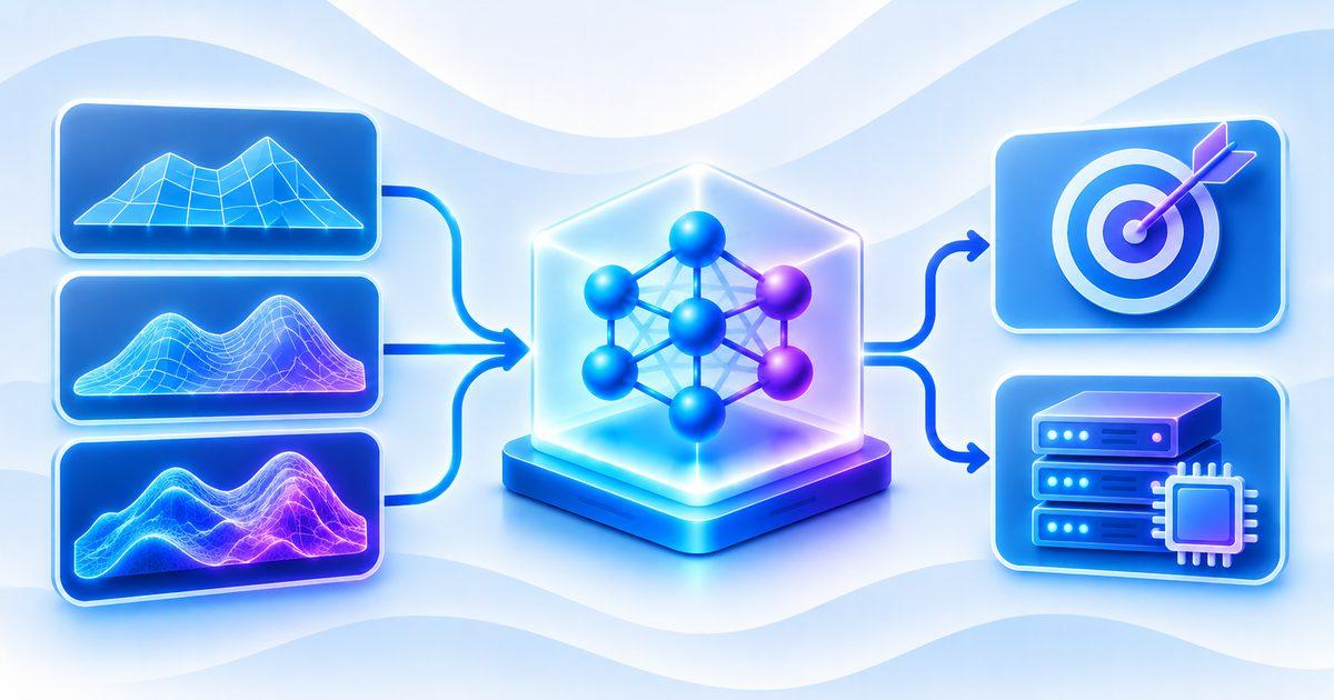
A neural operator is a machine learning architecture designed to learn mappings between spaces of functions rather than only mappings between individual finite-dimensional input and output vectors. This distinction is important because many engineering systems are naturally represented using continuous physical fields, such as velocity, pressure, temperature, density, and displacement.
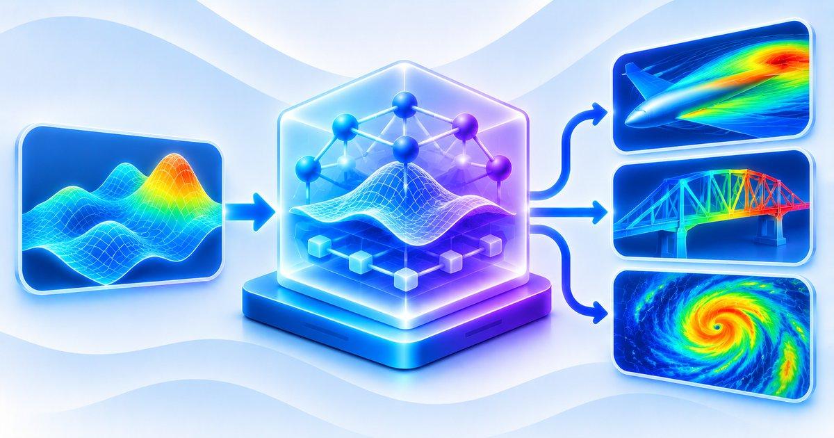
Consider a computational fluid dynamics problem involving airflow around an aircraft wing. The input conditions may include the wing geometry, incoming velocity field, fluid properties, and boundary conditions. The desired output may be the resulting pressure and velocity distributions across the computational domain. A conventional neural network might learn to predict an output for a fixed discretized representation of these inputs, whereas a neural operator aims to learn the underlying mapping between the input and output functions.
Mathematically, an operator can be represented as:
[
\mathcal{G}: a(x) \rightarrow u(x)
]
Here, (a(x)) represents an input function defined over a physical domain, while (u(x)) represents the corresponding output function. The operator (\mathcal{G}) describes how changes in the input function influence the resulting output field.
For example, an operator could learn how variations in an initial temperature distribution influence the temperature field after a specified period. Similarly, it could learn how different material properties and applied forces influence structural displacement.
The main advantage is that the model learns a family of physical relationships rather than memorizing individual simulation outputs. Once trained, it can evaluate new input conditions within its learned operating domain and potentially perform predictions at spatial resolutions different from those used during training.
This capability is valuable when engineering teams need repeated simulations. Instead of solving a computationally expensive PDE from scratch for every new configuration, a trained neural operator can provide a computationally cheaper approximation of the solution.
Traditional Numerical Solvers Versus Neural Operator-Based Approaches
Traditional numerical solvers approximate continuous physical equations by dividing the computational domain into discrete elements, grid points, or mesh structures. Engineers define the governing equations, establish boundary and initial conditions, select numerical discretization schemes, and solve the resulting system using appropriate computational algorithms.
Finite Difference Methods approximate derivatives using differences between neighboring grid points. Finite Element Methods divide complex geometries into smaller elements and use basis functions to approximate physical fields. Computational Fluid Dynamics uses numerical methods to solve equations governing fluid motion, including the Navier-Stokes equations.
These methods provide an important advantage: they are grounded in mathematical formulations of the underlying physical system. Their accuracy can be studied through numerical analysis, convergence properties, discretization error, and stability conditions. However, computational requirements can become substantial when simulations involve complex geometries, high-resolution meshes, nonlinear equations, or repeated parameter variations.
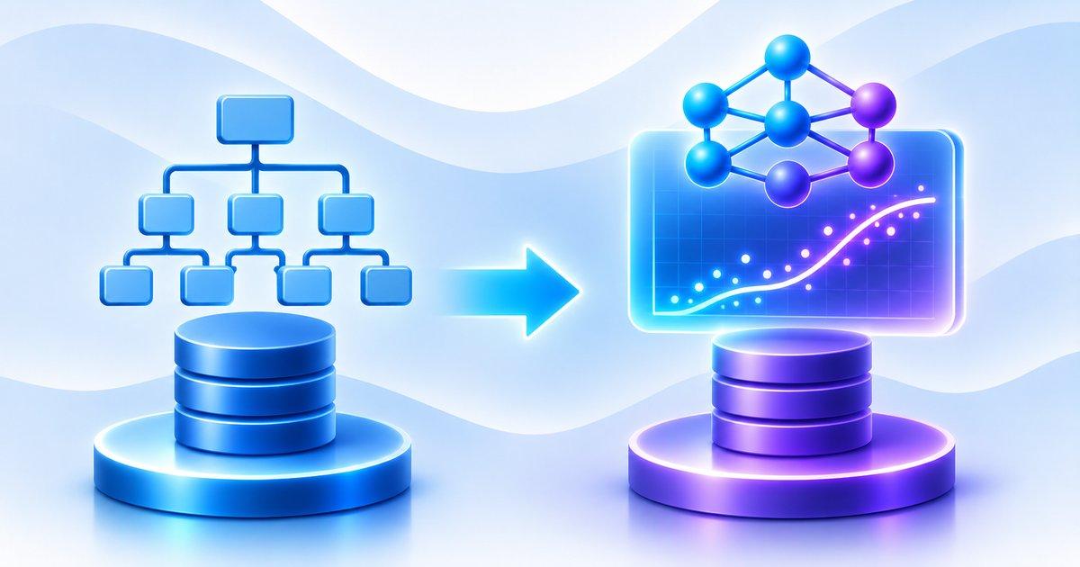
Neural operators introduce a learned approximation of the relationship between inputs and solutions. Rather than numerically solving every new problem from the beginning, they use patterns learned from previously generated simulation data or physics-informed training objectives.
For example, an engineering team might use a CFD solver to generate thousands of airflow simulations across different wing geometries and operating conditions. A neural operator can be trained on these input-output pairs and subsequently estimate airflow fields for additional configurations.
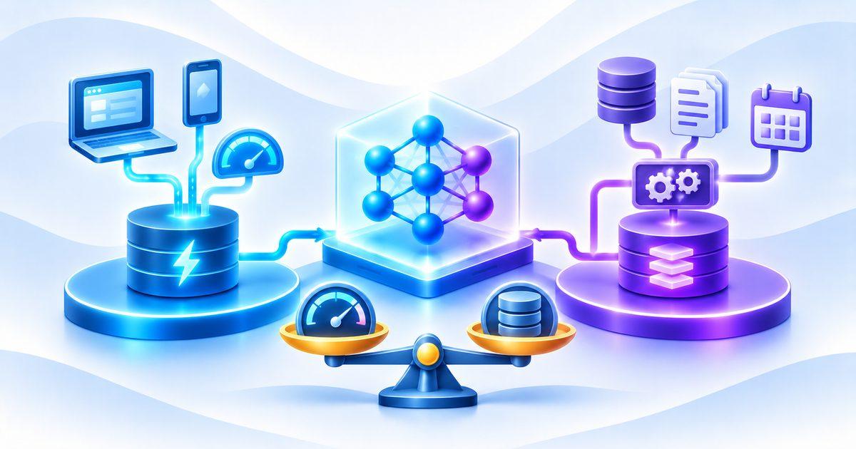
The important trade-off is that traditional solvers compute solutions through established numerical procedures, whereas neural operators approximate solutions using learned representations. The former generally offers stronger mathematical guarantees when properly formulated, while the latter may provide substantial inference speed advantages for repeated evaluations within the training distribution.
Neural operators should therefore be viewed as complementary computational tools. They are particularly useful for rapid prediction, parameter exploration, optimization, and surrogate modeling, while traditional solvers remain essential for generating reference solutions and validating critical engineering results.
Why Neural Operators Are Important for Scientific Machine Learning
Scientific machine learning combines machine learning techniques with mathematical modeling, scientific computing, and domain knowledge. Its objective is not simply to predict outputs from historical data but to improve how complex scientific and engineering systems are modeled, simulated, and optimized.
Neural operators are particularly relevant because they operate at the level of physical relationships. They can represent mappings between continuous input and output fields, which aligns naturally with the mathematical structure of many scientific problems.
One important capability is discretization flexibility. Traditional neural networks are often designed around fixed-size arrays or grids, while neural operators are developed to approximate mappings between function spaces. Appropriate operator architectures can therefore support evaluation on different discretizations, although practical implementations still have constraints related to interpolation, mesh structure, geometry, and numerical representation.
Another advantage is differentiability. Neural operators can provide differentiable approximations of physical solution processes, making them useful for inverse problems and engineering optimization. For example, a designer can investigate how changing material properties or geometric parameters influences a predicted physical outcome and use gradients to guide the optimization process.
Neural operators can also serve as surrogate models inside digital twins, where computationally efficient approximations are needed to represent physical systems under changing operating conditions.
For engineers interested in the data engineering foundation required to train such systems, "ML Data Pipelines for Software Engineers: From Event Streams to Model-Ready Data" provides relevant context on transforming raw observations and simulation outputs into structured machine learning datasets.
Key Takeaway
Neural operators extend deep learning beyond conventional input-output prediction by learning mappings between continuous function spaces. This makes them particularly useful for engineering systems governed by PDEs, where input conditions and resulting physical solutions are represented as spatial and temporal fields. Unlike traditional numerical solvers, neural operators learn an approximation of the solution process itself, enabling faster repeated predictions under suitable conditions. Their strongest applications emerge when combined with numerical simulation, physical knowledge, and reliable validation.
Section 2: Applying Neural Operators to Real-World Engineering and Scientific Problems
Computational Fluid Dynamics: Predicting Complex Fluid Flow
Computational Fluid Dynamics is one of the most important application areas for neural operators because fluid behavior involves complex spatial and temporal relationships. Engineers use CFD to understand airflow around aircraft, fluid movement through pipelines, turbulence in industrial equipment, and aerodynamic performance in automotive design.
Traditional CFD simulations solve the governing equations of fluid motion, particularly the Navier-Stokes equations. These equations describe the conservation of mass and momentum, with additional formulations accounting for energy and other physical properties where required.
The computational challenge increases when simulations involve turbulent flows, complex boundaries, high Reynolds numbers, and fine spatial resolution. Engineers may need to repeat simulations for different geometries, inlet velocities, pressures, or fluid properties, creating significant computational demands.
A neural operator can learn how changes in these input conditions influence the resulting velocity and pressure fields. Training data can be generated from CFD simulations covering different operating conditions and geometries. Once trained, the model can estimate flow fields for new configurations within the range of conditions it has learned.
For example, an automotive engineering team could train a neural operator using simulations of airflow around different vehicle designs. The model could provide preliminary estimates of pressure distribution and velocity fields, helping engineers compare design alternatives before performing more expensive simulations.
However, turbulence and other complex fluid phenomena introduce significant challenges. Small changes in initial conditions or geometry can influence flow structures, while important high-frequency features may be difficult to reproduce using a compressed representation. Models must therefore be validated using appropriate physical metrics, not only average prediction error.
Neural operators are particularly valuable for repeated CFD evaluations and design exploration, where a computationally efficient surrogate can reduce the time required to investigate multiple configurations.
Weather Forecasting and Climate Modeling
Weather and climate systems involve physical processes operating across multiple spatial and temporal scales. Atmospheric temperature, pressure, humidity, wind velocity, and other variables interact across large geographic regions, making numerical weather prediction computationally expensive.
Traditional forecasting systems use numerical models based on atmospheric physics and data assimilation. They solve complex equations using discretized representations of the atmosphere, requiring substantial computing resources to produce high-resolution predictions.
Neural operators provide an alternative way to learn mappings between atmospheric state variables and their future evolution. A model can be trained using historical observations or outputs from established numerical forecasting systems to predict future atmospheric fields.
For example, an operator model can learn how an initial atmospheric state evolves into a later pressure and wind distribution. The trained system can then provide rapid predictions for new initial conditions, potentially supporting faster forecasting workflows and ensemble experimentation.
However, weather forecasting requires careful treatment of physical conservation, uncertainty, and long-term stability. Small errors can accumulate during repeated prediction steps, and a model that performs well over short intervals may become unreliable over longer forecast horizons.
Climate modeling presents additional challenges because long-term behavior, rare extreme events, and interactions between atmospheric and oceanic processes must be represented accurately. Neural operators may complement existing numerical models by providing surrogate predictions for selected components or accelerating repeated scenario evaluation.
Their role should be determined by the required forecast horizon, physical constraints, and the availability of representative training data.
Digital Twins, Inverse Problems, and Engineering Optimization
Digital twins are computational representations of physical systems that can be updated using operational measurements, simulation outputs, and engineering models. They are used in manufacturing, energy systems, aerospace, infrastructure, and industrial operations to understand system behavior and support decision-making.
Neural operators can provide computationally efficient approximations within these digital twin environments. Instead of running an expensive physical simulation whenever operating conditions change, the digital twin can use a trained operator to estimate the resulting physical state.
Consider an industrial heat exchanger. Its performance depends on flow rate, temperature, pressure, material properties, and operating conditions. A neural operator trained on representative simulation data could estimate temperature and pressure distributions for different operating scenarios, helping engineers investigate performance changes more quickly.
Inverse problems offer another important application. In a forward problem, engineers provide physical parameters and calculate the resulting system behavior. In an inverse problem, they observe system behavior and attempt to infer the underlying parameters, material properties, or boundary conditions.
Because neural operators are differentiable, their predictions can be incorporated into optimization pipelines. Engineers can calculate gradients with respect to design parameters and use them to identify configurations that improve a desired objective, such as reducing drag, improving heat transfer, or minimizing structural deformation.
This capability can support design optimization by reducing the repeated computational cost associated with evaluating candidate designs. However, gradients from an approximate learned model may not perfectly represent the underlying physical system, so optimized configurations should be validated using trusted numerical solvers or physical experiments.
The adaptive nature of these systems is also important because operating conditions may change after deployment. Engineers can explore "Adaptive ML Systems: How Models Respond When the Environment Changes" to understand how models can be monitored and updated as the conditions represented by their training data evolve.
Key Takeaway
Neural operators have promising applications in computational fluid dynamics, weather forecasting, structural mechanics, materials science, digital twins, and engineering optimization. Their main advantage is the ability to approximate entire families of physical solution mappings, making repeated predictions more computationally efficient. However, different domains introduce different challenges involving turbulence, geometry, nonlinear material behavior, long-term stability, and physical constraints. Their most effective use is as validated computational surrogates that complement established numerical and experimental engineering methods.
Section 3: Engineering, Training, Evaluating, and Deploying Neural Operators
Building Training Datasets From Numerical Simulations and Physical Experiments
Training a neural operator requires datasets that represent relationships between input functions and their corresponding output functions. Unlike conventional supervised learning datasets containing individual feature vectors and labels, operator-learning datasets frequently consist of spatial fields, temporal observations, physical parameters, and solution representations.
Numerical solvers are commonly used to generate these datasets. For example, an engineering team developing a fluid simulation surrogate can use a CFD solver to generate velocity and pressure fields for different inlet conditions, geometries, and material properties. Each simulation produces an input configuration and a corresponding solution field that can be used as a training example.
The quality and coverage of the dataset are critical. If training simulations only represent a narrow range of operating conditions, the model may perform poorly when exposed to substantially different inputs. Engineers should sample relevant parameter ranges, boundary conditions, geometries, and initial states to capture the behavior expected during deployment.
Spatial discretization must also be considered. Training data may be generated on different meshes, grid resolutions, or coordinate systems. Depending on the architecture, these representations may require interpolation, coordinate normalization, mesh-aware processing, or function-based sampling.
Data pipelines must preserve the relationships between physical inputs and outputs. Inconsistent coordinate systems, incorrect boundary labels, missing simulation values, and differences in numerical solver configurations can introduce errors that undermine training.
The preprocessing workflow may include normalization, spatial alignment, temporal sampling, boundary-condition encoding, and feature construction. Engineers must also preserve the physical units and scaling relationships required to interpret the predictions correctly.
Teams building simulation-driven datasets can benefit from "Streaming Machine Learning: Building Models That Learn From Data in Real Time", particularly when engineering systems combine continuously collected measurements with historical simulation and experimental observations.
Training Neural Operators and Incorporating Physical Constraints
Training a neural operator generally involves minimizing the difference between predicted and reference output functions. The training process uses input-function and output-function pairs generated through simulations, measurements, or other validated sources.
A basic supervised objective can be expressed as:
\frac{1}{N}
\sum_{i=1}^{N}
\left|
\mathcal{G}_{\theta}(a_i)-u_i
\right|^2
]
Here, (\mathcal{G}_{\theta}) represents the neural operator, (a_i) represents an input function, (u_i) represents the corresponding reference solution, and (N) represents the number of training examples.
However, matching simulation outputs is not always sufficient. A model may achieve low average prediction error while violating physical relationships that are essential to the engineering application. Incorporating physics-based constraints can help address this issue.
For example, fluid-flow models may need to satisfy conservation of mass and momentum. Thermal models may need to respect energy conservation, while structural models may need to satisfy equilibrium relationships and boundary conditions.
A combined training objective can be written as:
\mathcal{L}{data}
+
\lambda_p\mathcal{L}{physics}
+
\lambda_b\mathcal{L}_{boundary}
]
Here, (\mathcal{L}{physics}) represents a physics-based residual, (\mathcal{L}{boundary}) measures violations of boundary conditions, and the coefficients control the relative contribution of each objective.
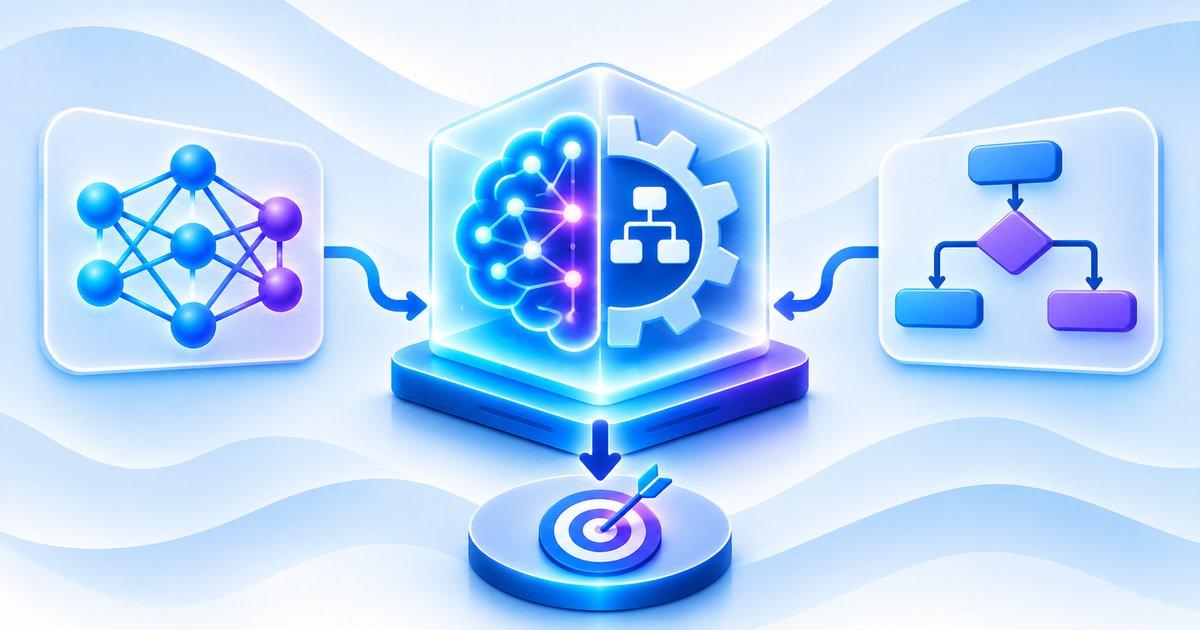
Physics-informed neural operators can therefore combine simulation data with mathematical constraints. Some architectures use PDE residuals during training, while others incorporate physical structure directly into their model representations.
The challenge is balancing these objectives. If physics-based losses dominate, the model may struggle to fit noisy or incomplete observations. If data-fitting losses dominate, it may produce predictions that match training examples but violate important physical properties.
Training strategies must therefore reflect the underlying equations, data quality, boundary conditions, and engineering objectives.
Evaluating Neural Operator Accuracy, Generalization, and Physical Reliability
Neural operator evaluation requires more than measuring the difference between predicted and reference fields. Engineers must determine whether a model generalizes across input conditions, spatial resolutions, geometries, and operating regimes while maintaining important physical properties.
Common numerical metrics include Mean Absolute Error (MAE), Root Mean Squared Error (RMSE), and relative (L_2) error. These measurements quantify the difference between predicted and reference solution fields, although their interpretation depends on the physical variables and their scales.
For example, a fluid simulation may need separate evaluation of velocity and pressure fields. A model can predict velocity accurately while producing significant pressure errors, or it may perform well on average while missing localized high-pressure regions.
Resolution generalization is another important evaluation dimension. A model trained on one discretization may be tested on a finer grid to determine whether it can provide useful predictions at a different resolution. Zero-shot super-resolution refers to evaluation at a finer resolution without retraining, but it should not be interpreted as guaranteed recovery of all missing physical detail.
Engineers should also evaluate out-of-distribution behavior. A model trained on moderate flow velocities may fail when exposed to substantially higher velocities or a different flow regime. Similarly, a structural model trained on a limited range of material properties may not generalize to materials with very different constitutive behavior.
Physical consistency metrics are equally important. These may include conservation-law residuals, boundary-condition errors, divergence constraints, energy balance, and stability across repeated prediction steps.
Uncertainty quantification adds another layer of reliability. An operator model should ideally indicate when an input condition is outside its reliable operating range, especially when predictions influence engineering decisions with safety or financial consequences.
Deploying Neural Operators Into Production Engineering and Scientific Computing Systems
Deploying a neural operator requires integrating model inference with the engineering software and computational infrastructure that already support simulation and analysis workflows. A production architecture may include simulation data pipelines, model training infrastructure, inference services, visualization tools, and connections to existing numerical solvers.
For example, an engineering design platform may allow users to modify geometry, material properties, or operating conditions. The application sends the updated configuration to a neural operator inference service, which estimates the corresponding physical solution fields. The results can then be visualized or passed to downstream engineering optimization components.
Model deployment can use GPU-based inference when computationally intensive architectures or large spatial fields are involved. CPU inference may be suitable for smaller models or applications where accelerator availability is limited. Engineers should benchmark the complete inference workflow rather than measuring only the time required for the neural network's forward pass.
Memory consumption can become a major concern when processing large spatial grids or three-dimensional physical fields. Batch size, resolution, model depth, and intermediate activation storage all influence deployment requirements. Efficient data movement and preprocessing can be as important as model architecture.
A hybrid deployment strategy can combine neural operators with conventional numerical solvers. The learned model provides fast estimates for routine design exploration, while selected configurations are validated through high-fidelity simulation. If the model encounters unfamiliar conditions or fails predefined reliability checks, the system can route the problem to a trusted numerical solver.
Production monitoring should track prediction errors whenever reference solutions or physical observations become available. Changes in operating conditions, geometry, sensor measurements, and material characteristics can cause model drift. Engineers should monitor these changes and establish retraining or recalibration procedures when performance deteriorates.
Ultimately, neural operators should be integrated into engineering workflows with clear validation requirements, model versioning, reproducibility, fallback mechanisms, and domain-specific acceptance criteria. Their computational advantages are meaningful only when the predictions remain sufficiently accurate and reliable for the intended engineering decisions.
Key Takeaway
Deploying neural operators successfully requires representative simulation datasets, physics-aware training, rigorous evaluation, and integration with existing engineering infrastructure. Models must be tested across different resolutions, geometries, operating conditions, and physical constraints rather than evaluated solely through average prediction error. Production systems should combine fast neural operator inference with trusted numerical solvers, uncertainty monitoring, and fallback mechanisms. This makes neural operators practical computational tools rather than unvalidated replacements for established scientific methods.
Conclusion
Neural operators represent an important development in scientific machine learning by extending deep learning to problems involving mappings between continuous functions. Instead of learning individual input-output predictions, they approximate the mathematical operators that connect physical conditions to resulting solution fields. This makes them particularly useful for engineering problems governed by partial differential equations, where repeated numerical simulations can require substantial computational resources.
Architectures such as Fourier Neural Operators, DeepONets, Graph Neural Operators, U-shaped Neural Operators, and Laplace Neural Operators demonstrate different ways of learning these relationships. Fourier-based models capture global spatial interactions, DeepONets provide flexible function-to-coordinate mappings, and graph-based approaches support irregular geometries and unstructured computational meshes.
The potential applications extend across computational fluid dynamics, weather forecasting, climate modeling, structural mechanics, materials science, digital twins, and engineering design optimization. By learning families of solution mappings, neural operators can accelerate repeated evaluations and provide differentiable approximations that support inverse problems and design exploration.
However, their effectiveness depends on more than neural network architecture. Representative simulation data, physical constraints, discretization handling, out-of-distribution generalization, uncertainty quantification, and numerical validation all influence whether predictions are suitable for engineering applications.
For software engineers and ML engineers entering scientific computing, neural operators introduce an opportunity to combine deep learning with numerical analysis and physical modeling. Their development requires understanding both machine learning systems and the mathematical structure of the engineering problems being solved.
The most practical direction is not to treat neural operators as universal replacements for CFD, FEA, or other numerical methods. Instead, they should be integrated as computationally efficient surrogates that accelerate selected workflows while preserving established numerical solvers for high-fidelity validation and critical engineering decisions.
As scientific machine learning continues to evolve, neural operators are likely to become increasingly important in simulation acceleration, digital twin development, and data-driven engineering optimization. Their ability to learn physical solution operators offers a promising path toward faster experimentation, more efficient design processes, and scalable computational engineering systems.
Frequently Asked Questions
1. What are neural operators in machine learning?
Neural operators are deep learning architectures that learn mappings between spaces of functions rather than only mappings between fixed-dimensional input and output vectors. They are particularly useful for modeling physical systems governed by partial differential equations, where inputs and outputs are continuous spatial or temporal fields.
2. How are neural operators different from traditional neural networks?
Traditional neural networks generally learn mappings between finite-dimensional representations, while neural operators aim to learn relationships between function spaces. This allows operator models to approximate families of physical solution mappings and potentially support different input and output discretizations.
3. What is operator learning in scientific machine learning?
Operator learning is the process of using machine learning to approximate mathematical operators that map input functions to output functions. It is commonly used to learn solution operators for differential equations and accelerate repeated scientific simulations.
4. What is a Fourier Neural Operator (FNO)?
A Fourier Neural Operator uses Fourier transforms to represent spatial information in the frequency domain and learn global relationships across physical fields. It has been applied to PDE problems involving fluid dynamics, Darcy flow, and other scientific simulations.
5. What is DeepONet, and how does it work?
DeepONet is a neural operator architecture containing branch and trunk networks. The branch network encodes the input function, while the trunk network encodes the output coordinates, and their representations are combined to estimate the resulting physical field.
6. What is the difference between FNO and DeepONet?
FNO learns spatial relationships through transformations in the Fourier domain, making it particularly suitable for structured spatial fields. DeepONet separates input-function encoding from output-coordinate encoding, offering flexibility when predictions are required at different or scattered locations.
7. Can neural operators solve partial differential equations?
Neural operators can approximate the solution operators associated with PDEs by learning from numerical simulations, experimental observations, or physics-informed objectives. They provide fast approximate predictions for new conditions within their learned operating domain, but they do not automatically guarantee the accuracy or stability of traditional numerical solvers.
8. What is the role of Fourier transforms in neural operators?
Fourier transforms convert spatial information into frequency components, allowing FNO architectures to learn global spatial interactions efficiently. Selected frequency modes are transformed and converted back into spatial representations to generate predictions.
9. How do graph neural operators handle irregular geometries?
Graph neural operators represent computational domains using nodes and edges that describe spatial locations and their connectivity. They use graph-based operations to learn physical relationships across unstructured meshes and geometries that are difficult to represent using conventional regular-grid methods.
10. How are neural operators used in computational fluid dynamics?
Neural operators learn relationships between fluid conditions, geometry, and resulting velocity and pressure fields. They can accelerate repeated CFD evaluations and support preliminary aerodynamic design exploration without requiring a complete numerical simulation for every configuration.
11. Can neural operators improve weather forecasting?
Neural operators can learn mappings between atmospheric states and their future evolution, potentially providing computationally efficient forecasts. Their reliability depends on physical consistency, training data coverage, forecast horizon, and the ability to generalize across changing atmospheric conditions.
12. What is the difference between neural operators and physics-informed neural networks?
Neural operators learn mappings between input and output functions, often representing solution operators across multiple physical conditions. Physics-informed neural networks generally approximate particular solutions while incorporating governing equations and physical constraints into their training objectives, although hybrid approaches combine both paradigms.
13. What are the main challenges of training neural operators?
Major challenges include generating representative simulation datasets, handling complex geometries, maintaining physical consistency, managing high-resolution spatial fields, and generalizing beyond training conditions. Engineers must also address computational requirements, uncertainty estimation, and numerical stability.
14. Can neural operators generalize to different spatial resolutions?
Certain neural operator architectures can support evaluation at resolutions different from those used during training. However, resolution generalization depends on architecture, discretization, boundary conditions, training coverage, and the physical scales represented by the model.
15. Are neural operators suitable for production engineering applications?
Yes, neural operators can support production engineering workflows as surrogate models for repeated simulation, design optimization, and digital twin applications. However, safety-critical decisions should incorporate physical validation, uncertainty monitoring, high-fidelity numerical solvers, and reliable fallback mechanisms.