Section 1: Understanding Event Time and Why Streaming ML Systems Get Time Wrong
Event Time, Processing Time, and Ingestion Time: Understanding the Differences
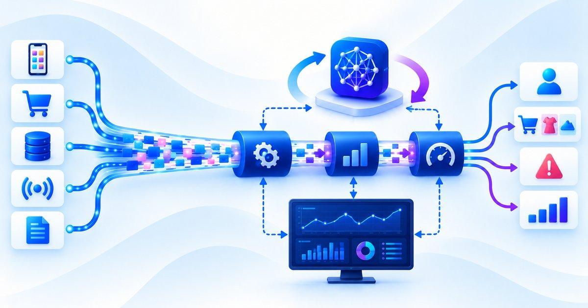
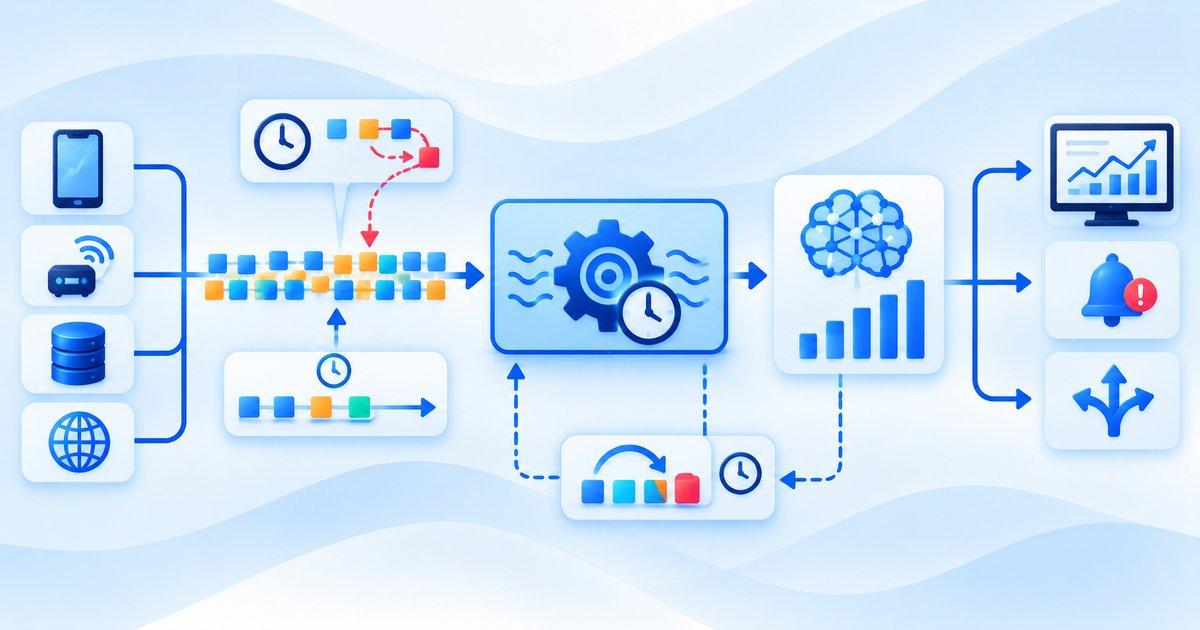
Real-time machine learning systems often make predictions using information that arrives continuously from applications, financial transactions, connected devices, application logs, and user interactions. Although these events are typically processed as they arrive, the moment an event reaches a processing system is not necessarily the moment the underlying activity occurred. A transaction may take several seconds to reach a data platform, a mobile device may remain offline for several minutes before uploading user activity, or a sensor may buffer measurements during a temporary network disruption, creating differences between when information becomes available and when the real-world event actually happened. These differences make time semantics a fundamental engineering concern because a streaming ML pipeline must determine which observations belong together, which information was available for a particular prediction, and whether a historical aggregate accurately represents the state of the world at that time.
Three timestamps are particularly important when designing these pipelines: event time, processing time, and ingestion time. Event time records when the source event occurred, according to the event's timestamp or source-defined clock, while processing time represents when a computation actually handles the event. Ingestion time generally refers to when the event enters a particular data system, such as a message broker or streaming platform, although its precise definition depends on the architecture. These timestamps may be close together in a low-latency system, but they can diverge significantly when networks are unreliable, queues become congested, or processing services experience uneven workloads. Engineering teams should therefore define each timestamp explicitly and avoid treating them as interchangeable fields.
Event-time processing becomes especially important when machine learning applications make predictions from continuously arriving information, because network delays and out-of-order events can cause the system to process incomplete or misleading representations of recent activity. The challenges discussed in “Streaming Machine Learning: Building Models That Learn From Data in Real Time” are closely related to this problem, since real-time ML systems must account for the timing of incoming observations while maintaining reliable predictions. By distinguishing event time from processing time and ingestion time, engineers can prevent delayed records from silently distorting time-sensitive features and prediction outcomes.
Why Events Arrive Late or Out of Order in Distributed Systems
Late and out-of-order events are normal characteristics of distributed data systems rather than exceptional conditions that can always be eliminated through faster infrastructure. Events may pass through mobile applications, local buffers, message brokers, network connections, multiple processing services, and storage systems before reaching the model, with each component introducing different delays or delivery guarantees. Parallel processing can also change arrival order because separate workers handle different partitions or batches at different speeds, meaning that an event generated earlier may be processed after another event generated later. Consequently, observing events in arrival order does not guarantee that they will be arranged correctly according to event time.
Mobile and edge devices introduce additional complications because they frequently operate with intermittent connectivity and limited opportunities to transmit data. A fitness tracker may collect heart-rate measurements throughout an underground commute but upload them only after connectivity returns, while an industrial sensor may buffer vibration readings during a gateway outage and transmit the accumulated events when the connection recovers. The resulting stream can contain a large group of historical observations alongside new measurements, which creates difficulties for windowed aggregations and time-sensitive predictions if the pipeline assumes that every event represents current activity. The challenge becomes more pronounced when historical events arrive in bursts, since a system must process the backlog without allowing recovery traffic to overwhelm ongoing production workloads.
Delivery mechanisms can also introduce duplicates, delayed messages, and inconsistent event ordering through retries and replay operations. For example, a producer may send an event successfully but fail to receive an acknowledgment, causing it to retry the transmission even though the original message has already been accepted by the downstream system. Similarly, replaying a historical topic to rebuild a feature table may place old events into a pipeline that is also receiving live traffic, requiring the application to distinguish historical recovery from current processing when appropriate. Robust designs combine event identifiers, idempotent processing, ordering policies, and explicit rules for late-arriving information so that delayed events can be handled without silently corrupting feature calculations.
How Network Delays, Retries, Clock Skew, and Mobile Devices Affect Event Ordering
Event-time processing depends on timestamp quality, but timestamps themselves can introduce errors when source clocks are inaccurate or inconsistent. Clock skew occurs when different devices or servers disagree about the current time, which may happen because of imperfect clock synchronization, configuration problems, or temporary loss of access to synchronization services. If two devices record related events using clocks that differ by several seconds, their timestamps may suggest an incorrect sequence even when the events were produced in the opposite order. Engineers must understand the clock behavior of each source and determine whether timestamps represent reliable event times, approximate local times, or values that require additional validation before they can be used for cross-system ordering.
Network latency further complicates this problem because delays can vary substantially from one event to the next, even when the same source sends all events through the same infrastructure. Congestion, retransmissions, broker partition imbalances, and temporary processing bottlenecks can cause newer events to arrive before older ones, while retries can amplify differences between event time and arrival time. A streaming pipeline that simply sorts events within a small processing-time interval may reduce some ordering problems but cannot guarantee correctness when delays exceed that interval. The appropriate strategy depends on the application’s latency tolerance, the expected delay distribution, the quality of source timestamps, and the consequences of acting on incomplete information.
In connected systems, these issues often occur together rather than independently, creating difficult scenarios for online feature computation. Imagine an autonomous monitoring application in which sensor measurements are generated on an edge device, buffered locally during a network interruption, and later transmitted through a gateway that retries failed requests. Some events may arrive late, others may be duplicated, and the local clock may have drifted during the interruption, leaving the processing service with an event sequence that is both incomplete and imperfectly timestamped. Addressing these conditions requires an explicit event-time model, reliable source metadata, sensible policies for duplicate detection, and validation of timestamp ranges, instead of relying on the assumption that arrival order provides a trustworthy representation of real-world chronology.
Key Takeaway
Event-time processing is essential for streaming ML systems because the time an event occurs, the time it enters a data pipeline, and the time it is processed can differ substantially. Network delays, distributed processing, retries, mobile-device buffering, and clock skew can all produce late or out-of-order data, affecting time-windowed features, historical training examples, and real-time predictions. By defining timestamp semantics, validating event metadata, managing duplicates, and preserving point-in-time correctness, engineering teams can build pipelines that handle temporal uncertainty without confusing event arrival order with the chronology of the underlying activity.
Section 2: Watermarks, Windows, and State Management for Event-Time Processing
Tumbling, Sliding, and Session Windows for Time-Based ML Features
Event-time windows allow streaming machine learning systems to organize continuously arriving events into meaningful periods based on when the underlying activities occurred rather than when the processing infrastructure happened to receive them. Many production ML features depend on time-bounded observations, including the number of transactions within five minutes, average equipment temperature over the previous hour, or frequency of failed authentication attempts during a recent interval. Without an explicit windowing strategy, engineers may calculate these features using arbitrary batches of arriving records, causing the resulting values to depend on network conditions and processing delays instead of representing the intended behavior. Event-time windowing provides a consistent framework for aggregating observations while establishing clear rules for when events belong together and how the resulting feature values should be updated.
Tumbling windows divide the timeline into fixed, non-overlapping intervals, such as consecutive one-minute or five-minute periods, with every event assigned to a single interval according to its event timestamp. This design is useful for calculations such as transactions per minute, hourly machine utilization, or the number of application errors generated within each reporting interval, because it creates clearly defined aggregation boundaries. However, a feature that measures activity over the most recent five minutes may need to reflect a continuously moving interval rather than the current fixed window, making tumbling windows less suitable when adjacent observations must contribute to overlapping feature calculations. Engineers should choose window boundaries based on the semantics of the feature rather than selecting an interval solely for implementation convenience.
Sliding windows address this requirement by recalculating aggregations over intervals that move forward at a defined step size, allowing a single event to contribute to multiple overlapping windows. For example, a fraud detection system might maintain a five-minute transaction count updated every 30 seconds, giving the model a more recent picture of transaction activity than a set of isolated five-minute buckets would provide. Session windows follow a different pattern by grouping related events separated by no more than a configured inactivity gap, making them useful for analyzing user sessions, browsing behavior, and sequences of application interactions whose duration varies. Each strategy introduces different computational and state-management requirements, so engineers must balance temporal resolution, feature usefulness, storage overhead, and the latency involved in updating the corresponding aggregations.
Watermarks and Allowed Lateness: Deciding When an Event-Time Window Is Complete
Event-time windows introduce an important question that cannot be answered merely by observing that the current clock has advanced beyond a window boundary: how can a streaming system determine whether additional events belonging to that window are still likely to arrive? Distributed systems cannot generally assume that all events appear in timestamp order, because network delays, buffered devices, retries, and uneven processing can cause historical records to arrive after newer observations. Watermarks address this challenge by providing a system's estimate of event-time progress, indicating that events earlier than a particular timestamp are no longer expected under the stream processor's current assumptions. A watermark is therefore an operational completeness estimate rather than an absolute guarantee that no earlier event will ever appear.
Consider a stream in which the latest observed event has an event timestamp of 10:12, while the system has already processed records associated with 10:10 and 10:11. If the configured watermark strategy estimates that events can typically arrive up to two minutes late, the processor may advance its watermark behind the latest observed event time rather than immediately declaring every earlier window complete. The exact calculation depends on the streaming framework and its configuration, but the underlying objective is to balance timely output against the likelihood that a window still has outstanding observations. A watermark that advances too aggressively can cause valid late events to be excluded from initial results, whereas a watermark that advances conservatively may retain state longer and delay outputs that downstream applications are waiting to consume.
Reliable event-time aggregation depends on how incoming records are ingested, validated, transformed, and organized before they reach downstream machine learning models, particularly when records arrive late or require historical corrections. The engineering practices discussed in “ML Data Pipelines for Software Engineers: From Event Streams to Model-Ready Data” provide relevant context for building pipelines that preserve event metadata, handle duplicate records, and maintain consistent transformations across streaming workloads. These capabilities help engineering teams apply watermarks, manage stateful aggregations, and define predictable policies for incorporating late-arriving events into model-ready features.
Managing Stateful Aggregations, Duplicate Events, and Late-Event Corrections
Streaming aggregations often require state because a model's features depend on information collected across multiple events rather than on each record independently. A system calculating the number of transactions associated with a customer over the previous hour, for example, must retain enough information to determine which events belong in the relevant time interval and when older observations should no longer contribute to the feature. Depending on the aggregation, state may contain running counts, sums, minimums, maximums, sketches, event identifiers, or the individual records needed to remove expired observations from a sliding window. Engineers must consider how state grows with event volume, how long it must remain available, and how the system restores it after failures without losing or double-counting previously processed information.
Duplicate events create a related challenge because message delivery and retry mechanisms may cause the same real-world activity to be represented more than once in the stream. If a transaction event is processed twice, a straightforward aggregation could increase the transaction count incorrectly, potentially causing a fraud model to interpret ordinary behavior as suspicious. Deduplication commonly relies on stable event identifiers or business keys, with the implementation retaining enough information to identify repeated records within the relevant retention period. The correct strategy depends on the uniqueness and stability of source identifiers, since two genuinely distinct events may share several attributes while a retried event may be identical to its original representation.
Late-event corrections add another dimension because previously calculated features may need to change after an event arrives outside the expected ordering interval. Suppose an equipment-monitoring pipeline computes the average vibration level for a one-minute window and initially produces a value before a buffered sensor reading arrives with an earlier event timestamp; incorporating that reading may change the average and alter the interpretation of the machine's condition. The system must determine whether to revise the stored aggregate, publish a correction, update a materialized feature, or leave the original value unchanged because the prediction or business action has already been finalized. Stateful stream processing therefore requires an explicit policy for both temporal expiration and historical revision, particularly when the same feature values are used by online inference, downstream analytics, and offline model training.
Key Takeaway
Reliable event-time processing depends on selecting appropriate windows, using watermarks to estimate the progress of event time, and explicitly defining how long late events may influence aggregation results. Stateful processing must also account for duplicate records, retained historical information, and corrections that can change previously calculated ML features. By balancing completeness against inference latency and establishing clear policies for preliminary, revised, and finalized outputs, engineering teams can build streaming pipelines that deliver useful predictions without silently treating arrival order as ground truth.
Section 3: Building Correct ML Features and Training Datasets From Late Events
Preserving Point-in-Time Correctness When Computing Streaming Features
Machine learning systems that consume streaming data must ensure that every feature represents the information that was legitimately available when a prediction was made, rather than the information that eventually became available after the underlying event occurred. This requirement, known as point-in-time correctness, becomes particularly important when late-arriving events can modify historical aggregates or when data pipelines reconstruct training examples from records that have been collected over an extended period. For example, a fraud detection model evaluating a payment at 10:05 should use the relevant transaction history available to the prediction service at that moment, rather than incorporating a transaction that occurred at 10:03 but did not arrive until 10:08. Although the delayed transaction belongs to the earlier event-time interval, including it in the original prediction's feature vector would introduce information that the model could not actually have accessed when making its decision.
Maintaining point-in-time correctness requires engineers to distinguish the time an event occurred from the time the event became available to the feature computation or prediction system. Event timestamps determine the temporal relationship between observations, while availability timestamps establish whether those observations could legitimately contribute to a historical prediction. When constructing a training dataset, the feature pipeline should reproduce this distinction by evaluating which records were available at each example's prediction timestamp and applying the appropriate event-time window boundaries. This approach prevents historical features from being silently reconstructed using information that arrived later, helping offline evaluation reflect the conditions the deployed model would encounter rather than an artificially complete view of the past.
Late events complicate this process because a corrected historical aggregate may differ from the value that was originally presented to a prediction service. A time-windowed transaction count, for instance, might initially include six transactions, but increase to seven after a previously delayed event arrives with a timestamp inside the same window. The corrected count may be appropriate for retrospective reporting or for a future prediction, but it should not automatically replace the historical feature value used to evaluate an earlier decision. Engineering teams must therefore preserve enough temporal and processing history to distinguish the feature's original value from its later corrected value, ensuring that training examples, prediction audits, and operational records remain consistent with the information available at each relevant point in time.
Keeping Online and Offline Features Consistent Across Late-Event Arrivals
Production machine learning architectures commonly calculate features through two related environments: online pipelines that supply low-latency predictions and offline pipelines that prepare historical datasets, analyze behavior, or support model training. The online system may maintain recent aggregates in a low-latency store, while the offline system processes larger collections of events to reconstruct historical feature values across millions of examples. Although these environments can use the same conceptual feature definitions, differences in timestamp interpretation, window boundaries, deduplication, late-event handling, and aggregation logic can cause them to produce different values for equivalent inputs. Such inconsistencies create training-serving skew, making it difficult to determine whether poor production performance results from the model itself or from differences between the features used during training and inference.
Consider a recommendation model that uses the number of product interactions generated by a user during the previous hour to estimate their current interests. The online pipeline might calculate the feature from events that have arrived and passed validation, whereas the offline pipeline might aggregate every event that eventually receives a timestamp within the relevant hour. If some interactions are uploaded late by mobile devices, the two systems can produce different counts even when both use the same nominal one-hour window. The discrepancy may persist across thousands of training examples, allowing the model to learn patterns based on more complete historical records than those typically available during live inference, which can make offline evaluation appear stronger than actual production results.
Late-arriving events can change historical aggregates, making it essential to preserve the distinction between the information available when a prediction was made and the information discovered afterward. Engineers can reduce training-serving skew by following the principles discussed in “Feature Stores Explained for Software Engineers: Managing ML Features Like Production Data”, particularly when coordinating feature definitions, historical retrieval, and online inference across different processing environments. Maintaining these relationships helps preserve point-in-time correctness and ensures that training examples do not incorporate information that would have been unavailable to the model during the original prediction.
Handling Delayed Labels, Historical Corrections, and Training-Data Leakage
Delayed data can affect labels as well as features, creating additional challenges for training supervised machine learning models. A feature describes the information available to the model when it makes a prediction, whereas a label represents the outcome the model is intended to predict, which may not become known until substantially later. In fraud detection, for example, a transaction may initially appear legitimate but receive a confirmed fraud label days or weeks after a customer reports the incident and an investigation concludes. Similarly, predictive maintenance systems may not know whether a sensor anomaly preceded a genuine equipment failure until an inspection or repair establishes the underlying cause, making label availability fundamentally different from event time.
Training pipelines must account for this delay when selecting examples and deciding whether their labels are sufficiently mature for model development or evaluation. Treating every unlabeled observation as a negative example can introduce systematic errors, especially when the missing label merely indicates that the outcome has not yet been confirmed. At the same time, evaluating a model against labels generated before the full observation period has elapsed can underestimate performance or distort comparisons between model versions, since recent examples may not have had enough time to produce observable outcomes. A more reliable approach defines an appropriate label-maturation period, records label availability and revision history, and excludes or separately handles examples whose outcomes remain unresolved under the evaluation policy.
Historical corrections can also introduce leakage when training datasets combine final outcomes with features reconstructed using future knowledge. Suppose a model predicts equipment failure from sensor readings available at 14:00, while a subsequent inspection at 16:00 identifies the failure and corrects several earlier maintenance records. Those corrections may improve retrospective analysis, but the original prediction must still be evaluated using the feature information available at 14:00 rather than the corrected dataset as it appears later. Engineers should establish separate temporal rules for feature eligibility and label selection, retaining the historical context needed to reproduce training examples and evaluate models fairly. By making the availability of both inputs and outcomes explicit, teams can avoid learning from information that would not have been accessible at prediction time while still incorporating delayed labels when they become appropriate for training.
Key Takeaway
Building reliable ML features from streaming data requires preserving the information that was available at each prediction timestamp, even when late-arriving events subsequently change historical aggregates or labels. Online and offline feature pipelines must share consistent definitions while retaining the temporal context needed to prevent training-serving skew, future-information leakage, and irreproducible evaluation. By versioning feature definitions and datasets, managing delayed labels explicitly, and separating retrospective corrections from point-in-time reconstruction, engineering teams can use late-arriving data to improve their systems without compromising the validity of model training and evaluation.
Conclusion: Building Reliable Machine Learning Systems With Event-Time Processing
Event-time processing is a foundational engineering capability for machine learning systems that make decisions from continuously arriving data, particularly when events are delayed, duplicated, or received in a different order from the sequence in which they occurred. Real-time applications depend on accurate temporal relationships to calculate transaction counts, behavioral indicators, equipment measurements, and other time-sensitive features, making timestamp interpretation an important part of the entire ML architecture. When a pipeline treats arrival time as a reliable representation of event chronology, it can generate incomplete aggregates, distort historical patterns, and produce predictions that differ from what the underlying data should support.
Reliable event-time processing begins by distinguishing event time, processing time, and ingestion time, since each timestamp describes a different stage in the lifecycle of an observation. Engineers must then choose appropriate windowing strategies, configure watermarks to estimate event-time progress, and establish allowed-lateness policies that determine how the system handles observations arriving after a window has advanced. Tumbling, sliding, and session windows support different feature requirements, while state management, deduplication, checkpointing, and replay help preserve consistent results as data continues to arrive. These mechanisms work together to make temporal behavior explicit, allowing the system to balance the need for timely predictions against the value of incorporating more complete information.
The implications extend beyond streaming infrastructure into feature engineering and model development, where the timing of information determines whether training examples accurately represent production conditions. Point-in-time correctness ensures that features used for a historical prediction contain only information that was available when that prediction would have been made, preventing late-arriving records from introducing future information into training or evaluation datasets. Online and offline feature pipelines must also follow compatible definitions for timestamps, aggregation windows, and data eligibility, while delayed labels require separate policies that account for when the true outcome becomes known. By preserving the distinction between original information availability and later historical corrections, engineering teams can improve data completeness without compromising the validity of model evaluation.
Production architecture must also account for the operational trade-offs created by late events, particularly when predictions influence decisions that cannot easily be reversed. A fraud detection service may need to respond immediately even when recent transaction history is incomplete, whereas a reporting pipeline may accept additional processing delay to improve aggregation completeness. Some applications can support preliminary results followed by corrections, while others need explicit rules for finalizing decisions and handling events received outside the accepted lateness period. The appropriate design depends on the application's latency requirements, the expected distribution of event delays, the cost of incorrect predictions, and the consequences of revising an earlier result.
Observability and testing make these policies dependable under real-world conditions by exposing changes in watermark lag, late-arrival rates, processing delays, feature distributions, and model performance. Engineers should validate out-of-order events, duplicate deliveries, historical backfills, checkpoint restoration, and recovery behavior, ensuring that unexpected arrival sequences do not silently corrupt state or create inconsistent outputs. Versioned feature definitions, explicit data contracts, reproducible processing logic, and controlled deployments further reduce the risk associated with changes to timestamp semantics and aggregation rules.
Ultimately, event-time processing should be treated as part of the machine learning system's correctness contract rather than as a configuration detail within the streaming platform. The goal is not to eliminate every late event, since distributed systems cannot guarantee that all data will always arrive promptly, but to define how temporal uncertainty affects features, predictions, and historical records. By combining appropriate windowing and watermark strategies with point-in-time correctness, reliable recovery, and comprehensive monitoring, engineering teams can build streaming ML systems that remain useful and trustworthy even when the data arrives late or out of order.
Frequently Asked Questions
1. What Is Event-Time Processing in Machine Learning?
Event-time processing is an approach to handling streaming data in which events are organized and analyzed according to when the underlying activity occurred rather than when the processing system received the records. It is particularly important for machine learning features based on recent transactions, user interactions, sensor measurements, and other time-dependent observations, because correct event-time interpretation helps preserve meaningful temporal relationships even when network delays or processing bottlenecks change arrival order.
2. What Is the Difference Between Event Time, Processing Time, and Ingestion Time?
Event time identifies when an event occurred according to the source timestamp, processing time records when a computation handles the event, and ingestion time generally describes when the event enters a particular system or processing boundary. These timestamps can differ because of network delays, buffering, retries, or processing congestion, making it necessary for engineers to define their semantics explicitly before using them to calculate time-windowed features or reconstruct historical training examples.
3. Why Do Events Arrive Late or Out of Order?
Events can arrive late or out of order because distributed systems process data across networks, message brokers, application services, and parallel workers that may introduce different delays. Mobile devices can buffer records while offline, producers may retry messages after communication failures, and uneven processing speeds can cause newer events to overtake older ones, making arrival order an unreliable representation of event chronology.
4. What Is a Watermark in Stream Processing?
A watermark is a mechanism for estimating how far event time has progressed in a streaming system and deciding when earlier windows can be treated as sufficiently complete for processing purposes. It helps balance timely results against the possibility of late-arriving events, but it does not guarantee that no older event will arrive after the watermark advances, so applications still need explicit policies for handling records that appear afterward.
5. What Is the Difference Between a Watermark and Allowed Lateness?
A watermark estimates event-time progress and helps the processor determine when to produce or advance window results, whereas allowed lateness defines how the application handles events that arrive after the relevant watermark has passed. Depending on the framework and configured policy, late events may update existing aggregates, produce revised outputs, be routed for additional processing, or be discarded, with the choice affecting data completeness, state retention, and prediction latency.
6. What Are Tumbling, Sliding, and Session Windows?
Tumbling windows divide event time into fixed, non-overlapping intervals, making them useful for calculations such as transactions per minute, while sliding windows use overlapping intervals to maintain measurements such as transaction counts over the most recent five minutes. Session windows group related events according to an inactivity gap, making them useful for variable-length user sessions or interaction sequences, with each strategy introducing different computational and state-management requirements.
7. How Does Event-Time Processing Improve Real-Time ML Features?
Event-time processing helps ensure that time-dependent features reflect the underlying chronology of observations rather than arbitrary variations in message arrival order. By assigning events to appropriate temporal windows and defining how late records affect aggregations, engineers can calculate more consistent features for applications such as fraud detection, anomaly monitoring, predictive maintenance, and behavioral modeling, even when data sources experience intermittent delays.
8. How Should Machine Learning Systems Handle Late-Arriving Events?
Systems should define an explicit late-event policy based on how much delay is acceptable and whether updated results remain useful to the application. Depending on the requirements, the pipeline may incorporate late events into existing state, publish corrected aggregates, process historical records through a separate reconciliation workflow, or reject events outside the accepted lateness period, while maintaining enough metadata to explain how each feature value was produced.
9. How Can Engineers Prevent Duplicate Events From Corrupting ML Features?
Engineers can reduce duplicate-processing errors by assigning stable event identifiers, maintaining suitable deduplication state, and designing aggregation updates to behave consistently when a message is processed more than once. These safeguards are especially important when producers retry transmissions, streaming jobs recover after failures, or historical events are replayed, because a duplicate transaction or sensor reading could otherwise inflate feature values and distort downstream predictions.
10. What Is Point-in-Time Correctness in Machine Learning?
Point-in-time correctness means that a feature vector represents only the information that was available to the model at the timestamp of the prediction being reconstructed or evaluated. This is essential when late-arriving records can change historical aggregates, because including a record that occurred earlier but arrived after the prediction would introduce information unavailable to the original model, potentially creating data leakage and overly optimistic offline evaluation results.
11. How Can Late Events Cause Training-Serving Skew?
Training-serving skew can occur when offline pipelines calculate historical features using all events eventually associated with a time window, while online services calculate features using only the records available at inference time. Delayed events can therefore produce different values for the same conceptual feature, allowing the model to learn from more complete historical information than it typically receives in production, which can reduce prediction quality even when the feature definitions appear identical.
12. How Should Systems Handle Delayed Machine Learning Labels?
Delayed labels should be managed according to when the outcome becomes sufficiently reliable for training or evaluation, rather than treating every currently unlabeled record as a negative example. Engineers should record label availability and revision history, establish appropriate maturation periods, and exclude or separately handle unresolved examples, ensuring that model comparisons are not distorted by outcomes that have not yet had enough time to become observable.
13. How Do Checkpointing and Replay Support Reliable Event-Time Processing?
Checkpointing preserves processing state and progress information so that a streaming application can recover from failures without unnecessarily rebuilding every intermediate result, while replay allows previously retained events to be processed again for recovery, historical backfills, or corrected computations. Both mechanisms require careful coordination with input positions, state restoration, and output publication, since recovery or replay can otherwise cause data loss, duplicate updates, or inconsistent historical aggregates.
14. Which Metrics Should Engineers Monitor in an Event-Time ML Pipeline?
Engineers should monitor watermark lag, late-arrival rates, event-time and processing-time differences, duplicate rates, queue depth, consumer lag, processing latency, and the frequency of corrected outputs to understand the temporal quality of incoming data. These measurements should be evaluated alongside feature distributions, prediction latency, and model outcomes when reliable labels become available, because a pipeline may continue operating normally while missing delayed events that are important to prediction accuracy.
15. How Can Organizations Choose the Right Event-Time Strategy for Production ML?
Organizations should choose an event-time strategy by evaluating prediction latency requirements, expected event-delay distributions, feature completeness, state-management costs, and the consequences of incorrect or revised decisions. Applications requiring immediate action may favor early predictions with controlled corrections, while workloads that prioritize complete historical aggregation may tolerate more delay, provided that the chosen watermark, lateness, recovery, and monitoring policies are tested against realistic production conditions.