Section 1: Understanding Liquid Neural Networks and Their Adaptive Architecture
What Are Liquid Neural Networks and Why Are They Different?
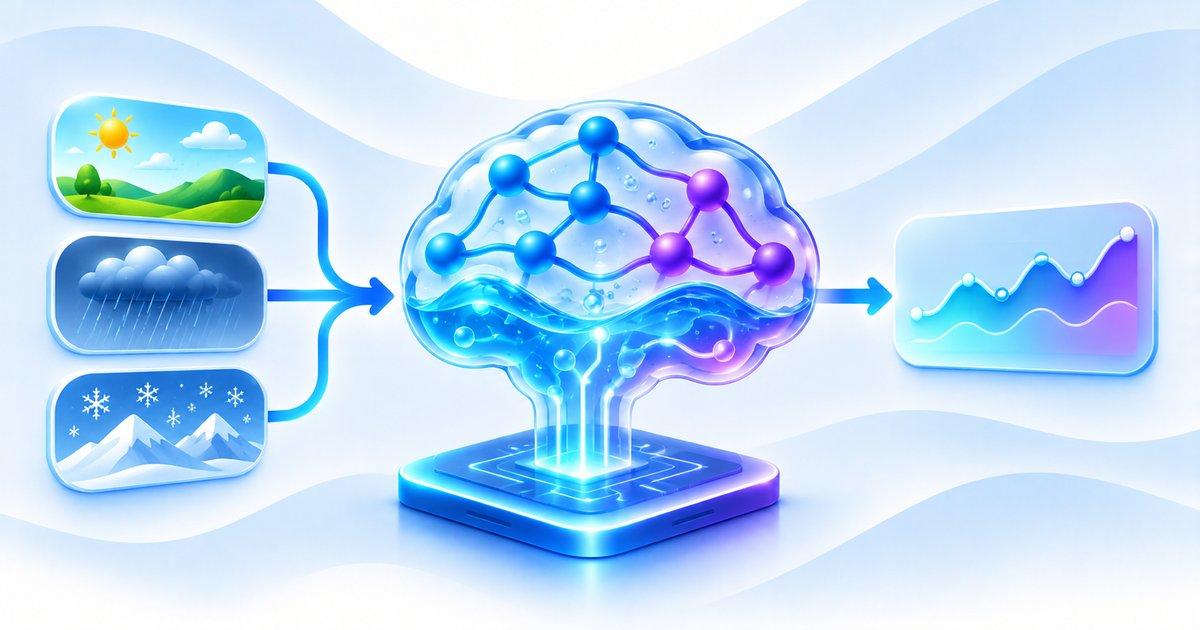
Liquid Neural Networks are a family of neural architectures designed to model continuously evolving information through dynamic internal states rather than relying exclusively on fixed computational transformations. Their distinguishing characteristic is the ability to change the effective timescales of internal state evolution according to incoming inputs and the current hidden state, allowing the network to respond differently as the conditions of a system change. This makes them particularly interesting for applications involving robotics, autonomous navigation, sensor monitoring, and other environments where information arrives continuously and the relationship between observations can evolve over time.
Conventional feed-forward neural networks generally apply a sequence of predefined mathematical transformations to their inputs, while standard recurrent neural networks maintain hidden states that are updated whenever a new observation arrives. Liquid neural networks extend the recurrent approach by representing hidden-state evolution through continuous-time dynamics governed by differential equations, allowing their internal behavior to depend on the current input and the state of the network. Instead of assuming that every observation should influence the system through an identical temporal response, the architecture allows effective time constants to vary according to learned interactions between inputs and internal states.
This characteristic becomes useful when a system encounters different operating conditions that require different temporal responses. An autonomous robot navigating a changing environment, for example, may need to respond quickly when an obstacle suddenly appears while retaining information about slower changes in its position, direction, and surroundings. A conventional model may also learn these relationships, but liquid architectures provide an explicit continuous-time mechanism for representing changing state dynamics, making temporal behavior a central component of the model design rather than simply treating observations as a fixed sequence of discrete updates.
Understanding Liquid Time-Constant Networks (LTCs)
Liquid Time-Constant Networks (LTCs) provide the mathematical foundation for an important class of liquid neural architectures by representing individual neurons as interconnected first-order dynamical systems whose behavior is influenced by nonlinear input-dependent signals. Each neuron maintains an internal state that evolves over time, with its rate of change determined by the incoming signals, recurrent connections, and learnable parameters.
A simplified LTC neuron can be described through the following continuous-time differential equation:
-\left[\frac{1}{\tau}+f(x(t),I(t),t,\theta)\right]x(t)
+
A f(x(t),I(t),t,\theta)
]
In this expression, (x(t)) represents the neuron's hidden state at time (t), while (I(t)) represents the external input received by the network. The parameter (\tau) represents a baseline time constant, (A) determines a reference state or activation level, and (f) represents a learned nonlinear function that depends on the current state, incoming signals, and trainable parameters. The important architectural property is that the nonlinear interaction influences the rate at which the hidden state changes, allowing the effective time constant to vary as the input and internal conditions evolve.
The effective time constant can be understood through the relationship:
\frac{\tau}{1+\tau f(x(t),I(t),t,\theta)}
]
This relationship illustrates why LTC neurons are described as liquid: their temporal responsiveness is not restricted to one fixed timescale, because the learned nonlinear interactions can influence how quickly internal states respond to changing inputs. During training, the model learns parameters that shape these dynamics through gradient-based optimization, while numerical differential-equation solvers calculate the state trajectories required for learning and inference. The resulting architecture provides a continuous-time representation of sequential information, although its computational cost depends partly on the numerical integration method and the complexity of the underlying dynamics.
Liquid Neural Networks vs. Traditional RNNs, LSTMs, GRUs, and Transformers
Liquid neural networks share their recurrent foundations with traditional RNNs, LSTMs, and GRUs, but differ in how they represent the evolution of internal states over time. A conventional RNN updates its hidden state through discrete computational steps, while LSTMs and GRUs introduce gating mechanisms that regulate how information is retained, modified, or discarded between observations. These gating mechanisms provide temporal flexibility, but their state updates generally follow discrete-time formulations in which each input advances the computation to another step. LTC architectures instead describe hidden-state evolution through continuous-time differential equations, with input-dependent dynamics influencing the effective timescales of individual neurons.
Transformers use a substantially different mechanism because self-attention allows tokens to interact with other positions in a sequence through query, key, and value representations. This provides powerful contextual modeling capabilities, particularly for language understanding and long-range relationships, but conventional dense attention introduces computational and memory requirements that increase with sequence length. Liquid neural networks approach sequential information through evolving recurrent states rather than constructing a complete attention relationship between sequence positions, making them interesting for certain applications involving continuous signals, changing temporal patterns, and irregularly sampled observations. Nevertheless, Transformers may remain more suitable for workloads requiring extensive contextual interactions, while established LSTM and GRU implementations may provide simpler and more mature solutions for many conventional time-series tasks.
Architecture selection should therefore depend on the actual characteristics of the application rather than assuming that continuous-time computation is inherently better than discrete-time processing. The broader discussion in “Adaptive ML Systems: How Models Respond When the Environment Changes” provides useful context for understanding why production environments introduce changing data distributions, evolving user behavior, and conditions that require ongoing model evaluation. Liquid neural networks offer one architectural approach to handling changing temporal inputs, but their usefulness must be established through comparisons involving predictive accuracy, inference latency, memory consumption, numerical stability, and performance under previously unseen operating conditions.
Key Takeaway
Liquid neural networks introduce continuous-time recurrent computation in which internal states evolve through input-dependent dynamics and effective time constants, allowing models to represent temporal information at different rates. Liquid Time-Constant Networks provide the mathematical foundation for this approach, distinguishing them from conventional RNNs, LSTMs, GRUs, and Transformer architectures through their differential-equation-based state evolution. For software engineers, the important distinction is that liquid networks adapt their internal dynamics to incoming information without automatically updating their learned weights, making them a promising architectural option for selected dynamic environments that must still be validated against established models and realistic application requirements.
Section 2: How Liquid Neural Networks Learn and Adapt Through Continuous-Time Dynamics
Understanding the Mathematics Behind Continuous-Time Neural Computation
The defining characteristic of liquid neural networks is their ability to represent hidden-state evolution through continuous-time differential equations rather than relying exclusively on fixed discrete-time updates. In conventional recurrent networks, a new observation typically triggers a hidden-state update according to a predefined computational step, whereas liquid time-constant models describe how internal states evolve over elapsed time in response to incoming signals and recurrent interactions. This mathematical formulation allows the network to represent temporal behavior at different rates, making it particularly relevant when observations arrive irregularly or the underlying system evolves continuously.
The hidden-state dynamics of an LTC network can be represented through a differential equation of the general form:
-\left[w_{\tau}+f(x(t),I(t),\theta)\right]x(t)
+
A f(x(t),I(t),\theta)
]
Here, (x(t)) represents the internal state of a neuron, (I(t)) represents the external input, (w_{\tau}) is a baseline decay-related parameter, and (A) represents a reference or reversal potential. The function (f) is a learned nonlinear transformation that depends on the current state, external input, and trainable parameters, allowing the neuron's state evolution to respond to changing information rather than following a completely fixed temporal pattern.
When multiple neurons are connected, their states influence one another through recurrent interactions, creating a network of coupled differential equations that jointly represent the evolving input signal. During training, the model's parameters are optimized through gradient-based learning, while numerical ODE solvers approximate the state trajectories required to calculate predictions and gradients. The choice of solver, integration interval, and numerical tolerance influences computational cost and the accuracy of the estimated trajectories, making numerical integration an important part of LTC implementation rather than an incidental software detail.
Input-Dependent Dynamics and the Role of Adaptive Time Constants
The adaptive behavior of liquid neural networks comes from the way their effective time constants depend on learned nonlinear interactions between incoming signals and internal states. Instead of forcing every neuron to respond at one fixed rate, the architecture allows the effective rate of state evolution to change as the input and recurrent activity change. A neuron processing a rapidly changing signal may therefore exhibit different temporal behavior from one responding to a slowly evolving pattern, allowing the network to represent multiple timescales within the same computational system.
Consider an industrial robot monitoring position sensors, motor currents, and vibration measurements while performing a repetitive operation. During normal movement, its sensor signals may change gradually, allowing the network to maintain a relatively stable internal representation of the robot's operating state, whereas a sudden vibration or unexpected movement may introduce a rapid change that alters the internal dynamics. Liquid neural networks can represent such changes through input-dependent state evolution, providing a mechanism for responding to evolving observations without requiring the same fixed temporal response for every input condition.
This property is also relevant when observations arrive at irregular intervals because the time elapsed between measurements can influence how the internal state should evolve. In many conventional sequence-processing pipelines, irregular observations are converted into fixed intervals through resampling, interpolation, or padding, which can introduce additional assumptions about the missing periods between measurements. Continuous-time models offer an alternative by incorporating elapsed-time information into state evolution, although engineers must still determine how timestamps, missing observations, and measurement quality are represented within the input pipeline. The challenges of handling asynchronous observations and delayed information are also discussed in “Event-Time Processing for Machine Learning: Handling Late and Out-of-Order Data”, which provides useful context for understanding why temporal information must be preserved when designing systems that process evolving data streams.
Importantly, adaptive time constants should not be confused with continuous parameter learning, because a trained liquid network can change its internal state trajectories in response to incoming information while retaining the same learned weights. Its adaptive behavior originates from the dynamics defined by the trained architecture rather than automatically updating the model through every new observation, making the distinction important when engineers compare liquid networks with online-learning or continual-learning systems.
Closed-form Continuous-time Networks (CfC): Reducing the Computational Cost
Although LTC networks provide expressive continuous-time representations, their reliance on numerical differential-equation solvers can introduce significant computational overhead during training and inference. Traditional numerical solvers approximate a state trajectory through repeated integration steps, with computational requirements influenced by solver choice, integration intervals, numerical tolerances, and the complexity of the underlying dynamics. These requirements can become expensive when networks process large datasets, long temporal sequences, or high-frequency sensor streams, motivating research into approaches that preserve liquid-style temporal behavior while reducing dependence on repeated numerical integration.
Closed-form Continuous-time Networks (CfC) were developed to address this computational challenge by approximating the dynamics of liquid time-constant systems through explicit time-dependent mathematical expressions. Rather than repeatedly applying a numerical ODE solver to calculate every state transition, CfC uses learned transformations and time-dependent gating mechanisms to produce state updates through a computationally efficient formulation. The approach builds on an approximate closed-form treatment of LTC dynamics, allowing the model to retain important continuous-time characteristics while avoiding the same solver requirements during its forward computation.
A simplified CfC update can be understood through an interpolation between two learned representations:
[
x(t)=
\sigma(-f(x,I,\theta_f)t)\odot g(x,I,\theta_g)
+
\left[1-\sigma(-f(x,I,\theta_f)t)\right]
\odot h(x,I,\theta_h)
]
In this expression, (f), (g), and (h) represent learned transformations, while the sigmoid term provides time-dependent gating that controls how the resulting representations are combined. The elapsed-time input influences the gating behavior, allowing the network to calculate state updates that reflect temporal differences between observations without requiring conventional iterative ODE integration for every update. The exact implementation includes architectural details and parameterizations beyond this simplified representation, but the equation illustrates how CfC makes time an explicit part of its computational mechanism.
The original CfC research demonstrated substantially faster training and inference in its evaluated continuous-time modeling tasks, while retaining expressive capabilities associated with liquid dynamics. However, CfC should be understood as an approximate computational formulation rather than a universally exact analytical solution to every possible LTC system, and its measured benefits depend on the task, architecture configuration, implementation, and hardware. Engineers should therefore compare solver-based LTC and CfC models using appropriate accuracy, latency, numerical behavior, and resource measurements before choosing between them for a production application.
Key Takeaway
Liquid neural networks use continuous-time differential equations to represent evolving internal states, with input-dependent dynamics allowing neurons to respond at different effective timescales as environmental conditions change. Liquid Time-Constant Networks provide the underlying dynamical formulation, CfC networks offer a computationally efficient approximation that reduces dependence on numerical ODE solvers, and Neural Circuit Policies introduce sparse connectivity structures that can make information flow easier to inspect. Understanding the differences between these mechanisms helps software engineers select appropriate architectures for irregular temporal data, robotics, and dynamic systems while accounting for numerical integration, computational efficiency, model structure, and the distinction between adaptive state evolution and actual online parameter learning.
Section 3: Real-World Applications of Liquid Neural Networks in Dynamic Environments
Robotics and Autonomous Navigation: Learning to Handle Unpredictable Conditions
Robotics and autonomous navigation represent important application areas for liquid neural networks because machines operating in physical environments must continuously interpret changing sensory information and respond to evolving conditions. Autonomous systems receive inputs from cameras, distance sensors, inertial measurement units, and other devices, with each observation providing information about the surrounding environment and the system's current state. Since these observations may arrive at different intervals and reflect rapidly changing conditions, liquid neural networks offer an interesting architectural approach through their input-dependent continuous-time dynamics, which allow internal representations to evolve according to incoming signals.
One notable research direction involves using liquid neural networks for autonomous flight navigation, where a controller must interpret visual information and generate appropriate control actions while operating under changing environmental conditions. Research published in Science Robotics demonstrated how a liquid neural network-based controller could support vision-based navigation in previously unseen environments, illustrating the potential of compact, adaptive neural dynamics for robotic systems. The architecture is particularly interesting because its internal state evolution can respond to incoming visual observations without requiring an increasingly large attention-based representation of the entire observation history, potentially supporting efficient processing in constrained robotic platforms.
In an autonomous drone, for example, a controller may receive camera observations while the vehicle encounters changing lighting, moving objects, different flight trajectories, and unexpected environmental disturbances. A liquid neural network can process these changing observations through evolving hidden states, allowing the internal representation to respond according to the current input and learned temporal dynamics. However, this capability does not guarantee safe navigation or successful obstacle avoidance under every condition, making environmental validation, sensor reliability, control constraints, and independent safety mechanisms essential components of a practical deployment.
Industrial IoT and Predictive Maintenance: Modeling Continuously Changing Equipment
Industrial environments generate continuous streams of operational information through sensors that monitor vibration, temperature, pressure, electrical current, rotational speed, and other equipment measurements. Traditional predictive maintenance systems often rely on statistical models or conventional recurrent architectures trained using historical operating data, but equipment behavior can change as machinery experiences different loads, operating temperatures, component degradation, and environmental disturbances. Liquid neural networks provide an alternative for representing these evolving temporal patterns because their internal states can adjust dynamically as incoming measurements change, potentially helping models capture relationships that occur across different timescales.
Consider an industrial motor operating under varying load conditions, where vibration measurements may gradually increase as components experience wear or change rapidly when an unexpected mechanical disturbance occurs. A liquid neural network can process these measurements through continuous-time state dynamics, allowing the model to represent both gradually evolving operational patterns and faster changes associated with unusual events. This capability may support applications such as equipment-state estimation, anomaly detection, predictive maintenance, and process monitoring, particularly when the timing between sensor observations varies or different signals evolve at different rates.
However, introducing liquid neural networks into industrial monitoring systems requires careful consideration of data quality, sensor calibration, temporal alignment, and the availability of reliable fault labels. A model trained primarily on normal operating conditions may still fail to recognize previously unseen equipment failures, while sensor noise, missing measurements, and changes in machine configuration can affect its predictions. Engineering teams should therefore compare liquid architectures against established time-series baselines such as LSTMs, GRUs, temporal convolutional networks, and state-space models, while evaluating detection quality, false alarms, inference latency, and performance across different operating conditions.
Healthcare Monitoring, Time-Series Analysis, and Human-Centered Applications
Healthcare monitoring provides another potential application area for liquid neural networks because physiological processes evolve continuously while medical observations are frequently collected at irregular intervals. Wearable devices and monitoring systems may generate heart-rate measurements, oxygen saturation readings, movement signals, temperature observations, and other physiological indicators at different sampling rates. Conventional time-series models often require these measurements to be resampled or transformed into fixed-length sequences, whereas continuous-time architectures provide an alternative approach for representing state evolution when observations arrive at varying intervals.
For example, a wearable monitoring system may collect physiological measurements throughout the day, with the frequency of observations changing because of device connectivity, battery constraints, or sensor availability. A liquid neural network could incorporate incoming measurements into its evolving internal state, potentially supporting applications involving patient-state estimation, physiological trend analysis, and personalized monitoring. Its ability to represent multiple temporal responses may be useful when a system must distinguish rapid changes in physiological signals from slower patterns that emerge over longer observation periods, although such capabilities require validation against clinically relevant datasets and established predictive models.
Healthcare deployment introduces particularly demanding requirements involving patient-level generalization, clinical validation, data privacy, uncertainty estimation, and the consequences of incorrect predictions. Physiological signals can vary substantially across individuals, medical conditions, age groups, and measurement devices, meaning that a model trained on one population may not perform reliably in another clinical setting. Liquid neural networks should therefore be evaluated against established approaches using carefully designed patient-level data splits, representative external validation datasets, and clinically meaningful performance measures, while maintaining human oversight and appropriate medical decision-making controls. The discussion of “Edge Machine Learning: How Engineers Run Intelligence Without the Cloud” is also relevant because wearable devices and connected monitoring systems may benefit from local inference when latency, connectivity, privacy, and computational constraints influence system design.
Key Takeaway
Liquid neural networks offer an interesting architectural approach for applications involving evolving physical environments, continuous sensor streams, and observations that arrive at irregular intervals. Research in robotic navigation demonstrates their potential for processing changing visual information, while industrial monitoring, edge robotics, and healthcare time-series analysis represent additional areas where continuous-time state evolution may provide useful modeling capabilities. However, successful deployment depends on representative data, reliable sensor infrastructure, numerical stability, hardware-specific benchmarking, rigorous validation, and independent safety mechanisms rather than assuming that adaptive internal dynamics automatically guarantee robust performance under every environmental condition.
Conclusion: Building Adaptive AI Systems With Liquid Neural Networks
Liquid Neural Networks represent an interesting development in deep learning because they introduce continuous-time state evolution as an alternative to conventional neural architectures that rely primarily on fixed discrete-time transformations. Through dynamically changing effective time constants, these networks can modify how their internal states respond to incoming information, allowing them to represent temporal patterns that evolve at different rates. This capability makes them particularly relevant to applications involving robotics, autonomous navigation, industrial monitoring, sensor processing, and other environments where observations arrive continuously and operating conditions change over time.
Liquid Time-Constant Networks provide the mathematical foundation for this approach by representing neuron behavior through differential equations whose dynamics depend on incoming signals, internal states, and learned parameters. Unlike conventional recurrent architectures that update hidden states through predefined discrete steps, LTC networks model how their internal representations evolve over elapsed time. This creates opportunities for processing irregularly sampled observations and modeling systems with changing temporal characteristics, although numerical integration, solver configuration, and computational stability remain important engineering considerations.
Closed-form Continuous-time Networks extend this direction by approximating liquid-style dynamics through computationally efficient closed-form updates, reducing dependence on repeated numerical differential-equation solving. Neural Circuit Policies introduce another complementary concept through sparse, biologically inspired connectivity structures that organize how sensory information flows toward intermediate processing layers and motor outputs. Understanding the differences between these approaches is essential because LTCs describe continuous-time state dynamics, CfC networks provide an alternative computational formulation, and NCPs define structured connectivity rather than representing interchangeable versions of the same architecture.
The potential applications of liquid neural networks extend across several dynamic environments, including autonomous flight, robotics, industrial equipment monitoring, edge AI, and physiological time-series analysis. Research involving vision-based robotic navigation has demonstrated the potential of liquid architectures for responding to changing environmental conditions, while industrial and healthcare applications offer additional opportunities for investigating continuous-time modeling. However, these applications require representative training data, rigorous validation, reliable sensor infrastructure, and appropriate safety mechanisms, particularly when model outputs influence physical systems or high-impact decisions.
For software engineers, the most important consideration is understanding what makes liquid neural networks adaptive without assuming that they automatically learn new parameters during every inference interaction. Their internal hidden states can evolve dynamically in response to incoming information while retaining the learned model weights, which is different from online learning or continual learning systems that explicitly update parameters. This distinction should guide architecture selection, system design, and expectations about how a deployed model will respond to changing conditions.
Ultimately, liquid neural networks should be evaluated as an additional architectural option rather than a universal replacement for LSTMs, GRUs, Transformers, or state-space models. Engineering teams should compare them against established baselines using representative workloads and measure predictive accuracy, generalization, inference latency, memory consumption, numerical stability, and hardware efficiency. By combining this evaluation with appropriate monitoring, fallback mechanisms, reproducible deployment configurations, and independent safety controls, organizations can determine whether liquid architectures provide meaningful advantages for the adaptive AI systems they intend to build.
Frequently Asked Questions
1. What are liquid neural networks?
Liquid neural networks are a family of neural architectures that model changing information through continuous-time dynamics and evolving internal hidden states. Their effective time constants can vary according to incoming inputs and internal network conditions, allowing them to represent temporal patterns that evolve at different rates. This makes them particularly interesting for applications involving robotics, sensor monitoring, autonomous systems, and irregularly sampled time-series data.
2. How do liquid neural networks differ from traditional neural networks?
Traditional feed-forward networks generally apply fixed sequences of mathematical transformations, while conventional recurrent networks update their hidden states through discrete computational steps. Liquid neural networks use continuous-time differential equations to describe how internal states evolve, allowing their effective temporal responses to change according to incoming information. This provides a different mechanism for modeling dynamic environments, although it does not automatically make liquid networks more accurate or computationally efficient than established architectures.
3. What are Liquid Time-Constant Networks (LTCs)?
Liquid Time-Constant Networks are continuous-time recurrent neural architectures in which individual neurons maintain internal states governed by differential equations. Their effective time constants can change through learned nonlinear interactions involving incoming inputs and existing hidden states, allowing neurons to respond at different temporal rates. LTCs provide the mathematical foundation for an important class of liquid neural networks and are commonly associated with applications involving evolving temporal signals.
4. How do adaptive time constants work in liquid neural networks?
Adaptive time constants influence how quickly an individual neuron's internal state responds to incoming information and evolves over time. In LTC architectures, learned nonlinear interactions between the external input and internal state influence the effective rate of state change, allowing the network to represent rapidly changing signals alongside slower temporal patterns. This mechanism provides temporal flexibility without requiring every neuron to operate at one fixed response rate.
5. Do liquid neural networks learn continuously during inference?
Liquid neural networks can adapt their internal hidden states continuously in response to incoming observations without necessarily updating their learned model parameters. Their adaptive behavior comes from the continuous-time dynamics established during training, rather than automatically modifying network weights whenever new information arrives. Actual online learning requires an additional learning mechanism that explicitly updates model parameters using new training information or feedback.
6. What is the difference between LTC and CfC networks?
Liquid Time-Constant Networks use differential equations to represent continuous-time hidden-state evolution, generally relying on numerical ODE solvers to calculate state trajectories. Closed-form Continuous-time Networks approximate liquid-style dynamics through computationally efficient mathematical updates, reducing the need for repeated numerical integration during execution. CfC networks can therefore offer practical computational advantages in selected workloads, although their accuracy and performance should be evaluated against appropriate LTC implementations.
7. What are Neural Circuit Policies, and how do they relate to liquid neural networks?
Neural Circuit Policies are sparse, biologically inspired network structures that organize information flow through groups of sensory, interneuron, command, and motor neurons. They can be combined with liquid-style dynamics to create architectures that process changing sensory inputs through structured recurrent connections. While LTCs describe how hidden states evolve and NCPs describe how neurons are connected, both can contribute different architectural properties to a neural control system.
8. How do liquid neural networks handle changing environments?
Liquid neural networks process incoming observations through internal states whose evolution depends on learned dynamics and the information being received. This allows the model to represent changes occurring at different temporal rates, potentially supporting applications where sensor readings, environmental conditions, and system behavior evolve continuously. However, the ability to adjust hidden-state dynamics does not guarantee robustness to every unfamiliar condition, making testing under representative and previously unseen environments essential.
9. Why are liquid neural networks useful for robotics and autonomous navigation?
Robotic systems frequently receive changing visual observations, sensor measurements, and movement-related information while operating under environmental uncertainty. Liquid neural networks provide a continuous-time recurrent mechanism for processing these observations through evolving internal states, potentially supporting navigation and control tasks where temporal behavior is important. Research involving vision-based flight navigation has demonstrated their potential, although practical deployment still requires independent safety controls, reliable sensors, and extensive environmental validation.
10. Can liquid neural networks work with irregularly sampled time-series data?
Liquid neural networks are particularly interesting for irregularly sampled time-series applications because their continuous-time formulation allows elapsed time between observations to influence internal-state evolution. Instead of assuming that every observation represents an identical fixed-duration interval, the model can incorporate temporal differences when calculating its evolving state. Engineers must still design appropriate timestamp handling, missing-data strategies, temporal preprocessing, and validation procedures to ensure that irregular observations are represented correctly.
11. Are liquid neural networks more efficient than LSTMs, GRUs, or Transformers?
Liquid neural networks can offer advantages for certain continuous-time and dynamic-environment workloads, but their efficiency depends on architecture configuration, numerical integration requirements, hardware, and implementation quality. Solver-based LTC networks may introduce additional computational overhead, while CfC formulations can reduce some of that overhead through approximate closed-form updates. LSTMs, GRUs, and Transformers may remain more practical for other applications because of their mature optimization libraries, established deployment tools, and strong task-specific performance.
12. What are the limitations of liquid neural networks?
Liquid neural networks introduce engineering challenges involving numerical integration, solver selection, training stability, temporal data preparation, and computational efficiency. Their predictive performance may also depend heavily on the quality of temporal observations and the representativeness of the conditions included during training. Additionally, their internal adaptive dynamics do not automatically provide online learning, guaranteed generalization, or safety under unfamiliar environmental conditions.
13. How are liquid neural networks trained and optimized?
Liquid neural networks are generally trained using gradient-based optimization methods that adjust the parameters controlling their continuous-time dynamics. LTC implementations calculate state trajectories through numerical differential-equation solvers, while CfC architectures use approximate closed-form updates that can reduce solver-related computational requirements. Training optimization involves selecting appropriate temporal representations, model configurations, numerical settings, regularization strategies, and validation procedures, with performance compared against established recurrent and sequence-modeling baselines.
14. Can liquid neural networks run on edge devices and embedded hardware?
Liquid neural networks may be suitable for selected edge and embedded applications because their recurrent state-based computation can avoid maintaining an expanding attention-based key-value cache. However, actual deployment efficiency depends on model size, numerical solver requirements, processor capabilities, memory availability, energy consumption, and inference implementation. Engineers should benchmark the complete model on the target hardware and evaluate whether it satisfies the application's real-time and resource constraints before selecting it for edge deployment.
15. Are liquid neural networks suitable for safety-critical production applications?
Liquid neural networks can be investigated for safety-critical applications involving robotics, autonomous systems, and industrial control, but their adaptive dynamics alone do not establish that they are sufficiently safe or reliable for deployment. Engineering teams must validate performance under unusual operating conditions, assess uncertainty and sensor failures, define output constraints, and maintain independent fallback controllers and emergency mechanisms. Applications involving physical systems or high-impact decisions should also include human oversight, reproducible testing, continuous monitoring, and formal safety evaluation appropriate to the deployment environment.